Quck Start

Drawing figures and plots with the GLE language is easy. A GLE file is a collection of drawing commands that the GLE program converts into either a bitmap or vector graphics file.

Language details

GLE is NOT case sensitive.
It does NOT require a special character to terminate the line
Commands cannot be broken over multiple lines
The first drawing command must be a size command to define the figure size
Distances are measured in centimeters and angles in radians
The origin is at the lower left part of the figure
! is the comment character. All text after it is ignored.
Data for a plot is contained within a separate file from the GLE script.
Drawing occurs at the current point that is changed with absolute amove x y and relative rmove x y commands.
The initial current point is (0,0) at the lower left corner.
The graphics state such as line widths colors, styles, fonts can be retained and restored with the gsave and grestore commands.

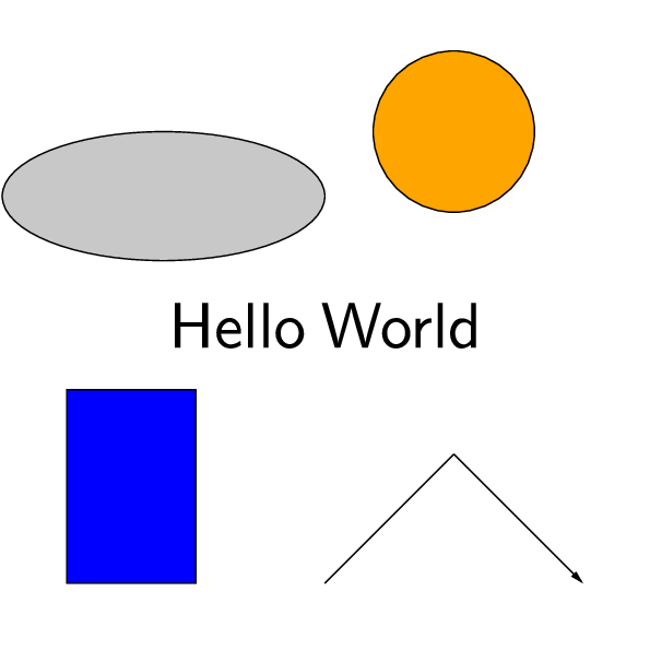
Hello World Example

A drawing of some basic shapes and text.

hello_world.gle

size 10 10
set font texcmss
set hei 1.0
amove 1 1
box 2 3 fill blue
rmove 6 7
circle 1.25 fill orange
amove 5 5
set just cc
write "Hello World"
amove 5 1
rline 2 2
rline 2 -2 arrow end
amove 2.5 7
ellipse 2.5 1 fill gray10

hello_world.gle

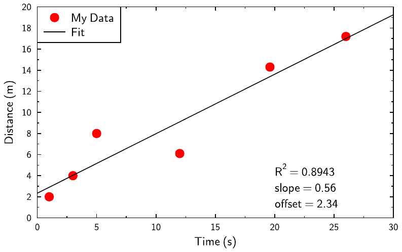
Plotting Data

A plot of data that is contained in a separate text file and fit to a straight line.

Create a plain text file called data.csv that contains some data, which may look like

! sample scatter plot data
1,2
3,4
5,8
12,6.1
19.6,14.3
26,17.2

Create a gle file called ascatterplot.gle that exists in the same folder as data.csv that loads the data and draws a plot.

ascatterplot.gle ascatterplot.zip zip file contains all files for this figure.

ascatterplot.gle

!
!  ascatterplot.gle - A scatter plot - plots data contained in data.csv and fits it with a straight line
!
size 10 10/1.6

set font texcmss
set hei 0.3
amove 0 0
begin graph
    scale auto
    data "data.csv" d1 = c1 , c2
    d1 marker fcircle color red key "My Data"
    let d2 = linfit d1 myslope myoffset myR2
    d2 line color black key "Fit"
    xtitle "Time (s)"
    ytitle "Distance (m)"
    key compact position tl
end graph
! display information on the graph
amove xg(20) yg(3)
write "R^2 = "+format$(myR2,"fix 4")
rmove 0 -0.3
write "slope = "+format$(myslope,"fix 2")

data_plot.gle

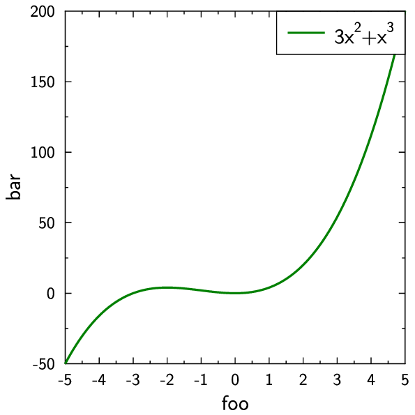
Plotting a function

GLE can plot mathematical functions and comes with standard mathematical functions, constants, and several special functions built in.

function_plot.gle

!
! -- function_plot.gle example of plotting a function
!
size 10 10
set font texcmss
set hei 0.5
amove 0 0 
begin graph
    scale auto
    let d1 = 3*x^2+x^3 from -5 to 5 nsteps 1000
    d1 line color GREEN lwidth 0.05 key "3x^2+x^3"
    xtitle "foo"
    ytitle "bar"
end graph

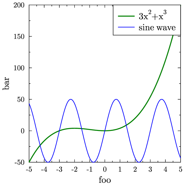
Custom functions and subroutines can be written as shown below, where pi is an understood constant.

user_function_plot.gle

!
! -- user_function_plot.gle example of plotting a user defined function
!
size 10 10
set font texcmr
set hei 0.5
amove 0 0
sub my_function x b c
    return b*sin(2*pi*x/c)
end sub
begin graph
    scale auto
    let d1 = 3*x^2+x^3 from -5 to 5 nsteps 1000
    d1 line color GREEN lwidth 0.05 key "3x^2+x^3"
    let d2 = my_function(x,50,3) from -5 to 5 nsteps 1000
    d2 line color BLUE lwidth 0.03 key "sine wave"
    xtitle "foo"
    ytitle "bar"
end graph