SPM Images

Scanning Probe Microscopy (SPM) Images

AFM.gle

!-----------------------------------------------------------------!
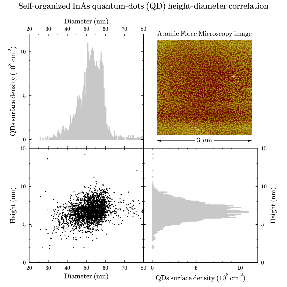
!   These graphs illustrate the correlation of the heights and di-!
! ameters of a set of InAs self-organized quantum-dots (QD), grown!
! over GaAs by means of Molecular Beam Epitaxy.                   !
!   The figure was obtained by means of Atomic Force Microscopy.  !
! The histograms was obtained from the figure by counting and     !
! measuring the height and diameter of each quantum-dot (each     !
! circle). The correlation gives rise to what is known as quantum-!
! dots families.                                                  !
!                                                                 !
! Author:  Ivan Ramos Pagnossin                                   !
! Data:    December 2003                                          !
! Project: Master thesis                                          !
!-----------------------------------------------------------------!

size 15 15

set font texcmr

! Graph at the lower left corner.
amove 1.5 1.25
begin graph
   size 6 6
   fullsize
   xaxis min 20 max 80 dticks 10 dsubticks 5
   yaxis min 0  max 15 dticks 5  dsubticks 1
   xtitle "Diameter (nm)"
   ytitle "Height (nm)"
   ! Quantum dots (QD) diameter-height correlation data.
   data "3um/3um-diameterXheight.dat"
   d1 marker fcircle msize 0.05
end graph

! Graph at the upper left corner.
amove 1.5 7.25
begin graph
   size 6 6
   fullsize
   xaxis min 20 max 80 dticks 10 dsubticks 5
   yaxis min -1 max 12 dticks 5  dsubticks 1
   xlabels  off
   x2labels on
   x2title "Diameter (nm)"
   ytitle "QDs surface density (10^8 cm^{-2})"
   ! Quantum-dots (QD) diameter distribution.
   data "3um/3um-diameter.dat"
   bar d1 width 0.4 color grey10 fill grey10
end graph

! Graph at the lower right corner.
amove 7.5 1.25
begin graph
   size 6 6
   fullsize
   xaxis min -1 max 12 dticks 5 dsubticks 1
   yaxis min 0  max 15 dticks 5 dsubticks 1
   ylabels  off
   y2labels on
   xtitle "QDs surface density (10^8 cm^{-2})"
   y2title "Height (nm)"
   ! Quantum-dots (QD) height distribution.
   data "3um/3um-height.dat" 
   bar d1 horiz width 0.1 color grey10 fill grey10 
end graph

! Atomic-force microscopy image at the upper right corner.
amove 8.2 7.95
begin name img
   bitmap "3um/3um.png" 5 5
end name

set just cc
amove ptx(img.tc) pty(img.tc)+0.3
write "Atomic Force Microscopy image"

amove ptx(img.bl) pty(img.bl)-0.3
aline ptx(img.br) pty(img.br)-0.3 arrow both
amove ptx(img.bc) pty(img.bc)-0.3
begin box add 0.1 nobox fill white
   tex "3 $\mathrm{\mu m}$"
end box

set hei 0.45
amove 7.5 14.7
write "Self-organized InAs quantum-dots (QD) height-diameter correlation"

bitmap.gle

! Demo about importing bitmaps.
! Author: Francois Tonneau

! Original script, bitmap, and figure by Ivan Ramos Pagnossin.

size 18 10

! ==========

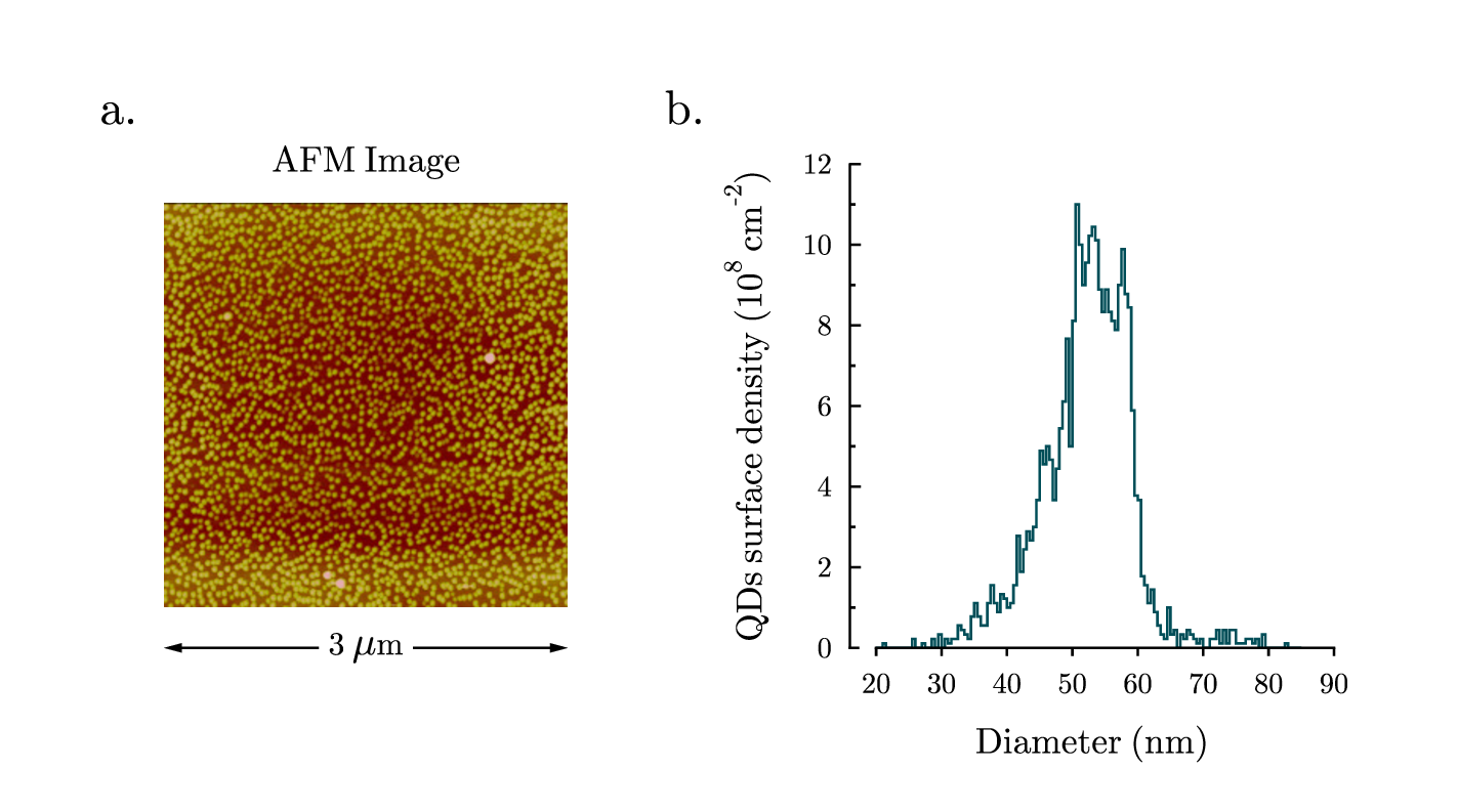
! Our figure has two panels. We start with panel (a).

set font ss hei 0.60 just bl
amove 1.2 8.5
write "a."

! We use the 'bitmap' command to import the 'bitmap.jpg' file into the figure.
! The name of the image file is 'bitmap.jpg', and the resulting image will have
! a width of 5 cm. A nominal height of 0 tells GLE to respect the aspect ratio
! of the bitmap file. The import is done within a 'begin name ... end name'
! block to be able to refer to the image by name:

amove 2.0 2.5
begin name afm_image
   bitmap "bitmap.jpg" 5 0
end name

! Now that the image has been named ('afm_image'), we can refer to the 'afm_image'
! region and its reference points (e.g, 'tc': top center; 'bl': bottom left).
! We can also locate their position via the ptx() and pty() functions.

set hei 0.45 just cc
amove ptx(afm_image.tc) pty(afm_image.tc)+0.5
write "AFM Image"

set lwidth 0.03
amove ptx(afm_image.bl) pty(afm_image.bl)-0.5
rline 5 0 arrow both
rmove -5/2 0
begin box add 0.1 fill white nobox
   write "3 \sethei{.50}\mu \sethei{0.4}m"
end box

! ==========

! We now turn to panel (b), which is a line plot in the 'hist' step style.

set font ss hei 0.60 just bl
amove 8.2 8.5
write "b."

set hei 0.45

amove 10.5 2.0
begin graph
    size 6 6
    fullsize
    xaxis min 16 max 90 ftick 20 dticks 10
    yaxis min 0 max 12 ftick 0 dticks 2
    xside     off
    x2axis    off
    y2axis    off
    xsubticks off
    xticks length -0.1
    xtitle "Diameter (nm)" dist 0.4
    ytitle "QDs surface density (10^{8} cm^{-2})" dist 0.4
    data "bitmap.dat"
    d1 line hist color #004e58
end graph

! We cover the axes with solid lines as a finishing touch:

set cap square
amove xg(20) yg(0)
aline xg(90) yg(0)

amove xg(16) yg(0)
rline 0.1 0

! Done. We have learned to import bitmap images in GLE.

inpstm.gle

!
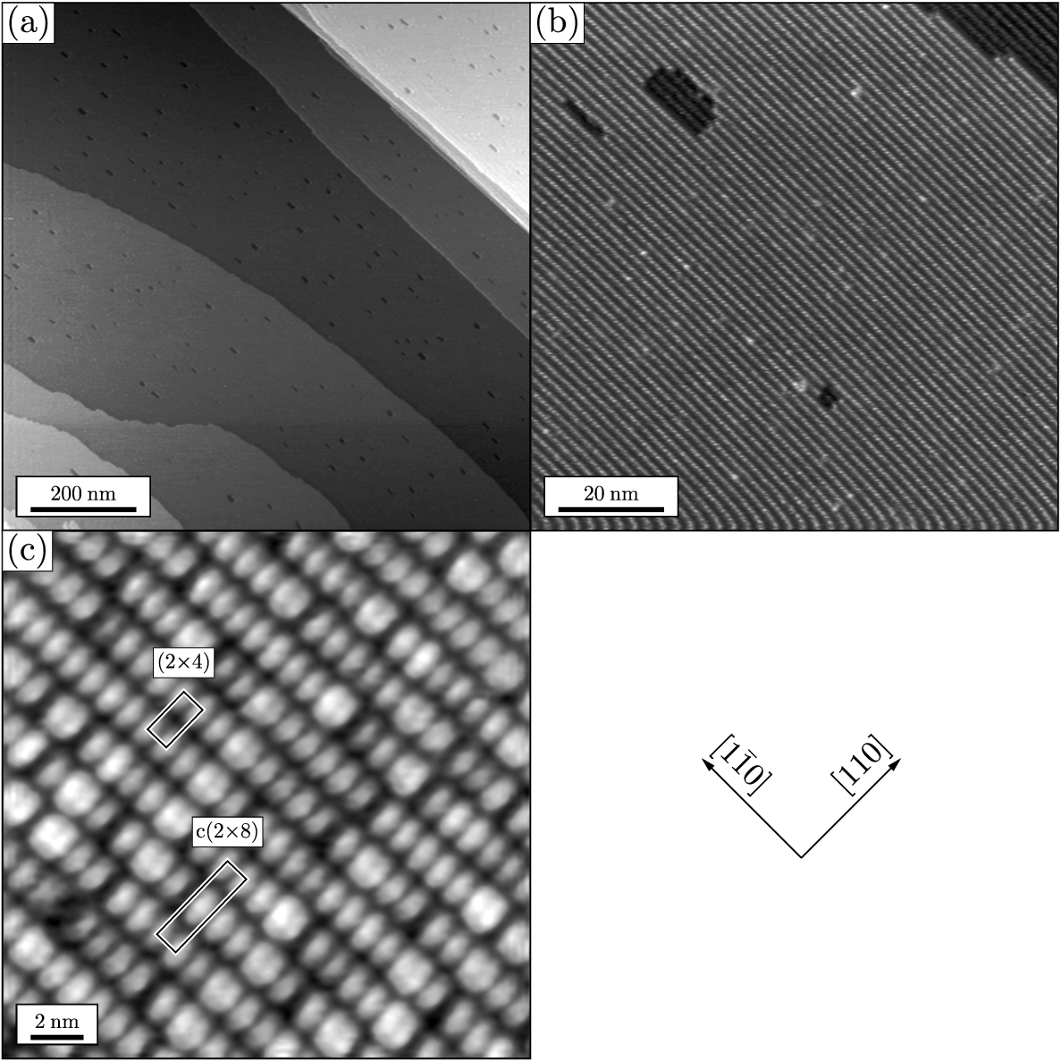
! InP(001) STM images three images of the (2x4)/c(2x8) reconstruction
! example of how to layout three STM images
! By: V.P. LaBella vlabella@albany.edu
! the eps output of this gle file was submitted directly
! to the journal.  See Figure 2 in The Jour. Vac. Sci. & Technology A, Vol. 18 no. 4 pp. 1492 (2000)
! be sure to get the stm.gle include from the GLE function repository
!
size 15 15

include stm.gle

set font ss hei 0.5

dx = 15; dy = 15
idx = dx/2; idy = idx

tbox = idx/2-0.5
scale_bar_x = 0.2
scale_bar_y = 0.2

!
! 1000 nm x 1000 nm (2x4)
!
amove 0 idy
box idx idy
bitmap "tiff/large.png" idx idy
@textbox 0 2*idy "tl" 0.5 "(a)" 0.05 0.1 1 "WHITE" "BLACK" "BLACK" 0.01
@scale_bar idx/1000*200 0.3 "200 nm" scale_bar_x idy+scale_bar_y "lr" 0.07 0.1 "WHITE" 1 0.2 0.1

!
! 100 nm x 100 nm (2x4)
!
amove idx idy
box idx idy
bitmap "tiff/med.png" idx idy
@textbox idx 2*idy "tl" 0.5 "(b)" 0.05 0.1 1 "WHITE" "BLACK" "BLACK" 0.01
@scale_bar idx/100*20 0.3 "20 nm" idx+scale_bar_x idy+scale_bar_y "lr" 0.07 0.1 "WHITE" 1 0.2 0.1

!
! 20 nm x 20 nm (2x4)
!
amove 0 0
box idx idy
bitmap "tiff/small.png" idx idy
@textbox 0 idy "tl" 0.5 "(c)" 0.05 0.1 1 "WHITE" "BLACK" "BLACK" 0.01
@scale_bar idx/20*2 0.3 "2 nm" scale_bar_x scale_bar_y "lr" 0.07 0.1 "WHITE" 1 0.2 0.1

!
! draw the direction arrows
!
axis_l = 2.0
@axis_box 1.5*idy 0.5*idy-1.0  "[110]" "[1\={1}0]" 45 0.1 0.1 axis_l "cc" 0 "BLACK" "WHITE" "BLACK" 0.45 0.1

!
! That's it!
! All the STM images are in place with the proper scales and labels.
!
! Now draw some text over the images
! to identify the unit cell
! 2x4 box
!

a = 0.7*idx/20

by2 = 2*sqrt(2)*a/2
by4 = 2*by2; by8 = 2*by4-0.04
line1 = 0.07
line2 = 0.02
angle = 46

! 2x4 box
amove 2.328 4.419
begin rotate angle
    set lwidth line1 color white
    box by4 by2
    set color black lwidth line2
    box by4 by2
end rotate
xp = xpos()+by4*cos(torad(angle))-by2*sin(torad(angle))
yp = ypos()+by4*sin(torad(angle))+by2*cos(torad(angle))+0.2
@textbox xp yp "bc" 0.3 "(2\times 4)" 0.05 0.1 1 "WHITE" "BLACK" "BLACK" 0.01

!2x8 box
amove 2.461 1.508
begin rotate angle
    set lwidth line1 color white
    box by8 by2
    set color black lwidth line2
    box by8 by2
end rotate
xp = xpos()+by8*cos(torad(angle))-by2*sin(torad(angle))
yp = ypos()+by8*sin(torad(angle))+by2*cos(torad(angle))+0.2
@textbox xp yp "bc" 0.3 "c(2\times 8)" 0.05 0.1 1 "WHITE" "BLACK" "BLACK" 0.01