Color Maps

Charts using color to depict values or false color maps.

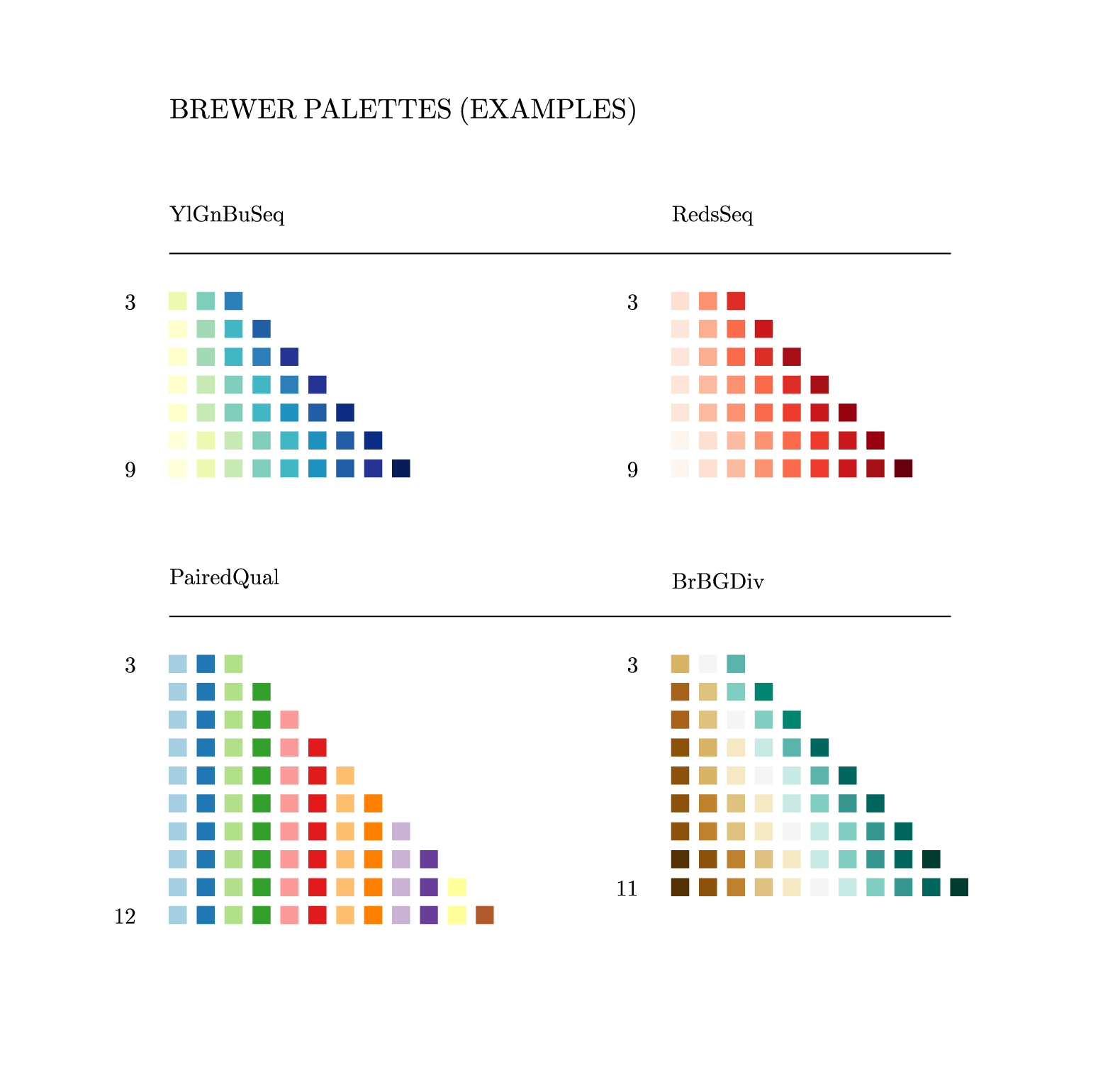
brewersample.gle

brewersample.gle brewersample.zip zip file contains all files for this figure.

brewersample.gle

! A small sample of Brewer palettes.
! Author: Francois Tonneau

include brewer.gle

size 20 19

set font ss hei 0.5 just bl

amove 3 16.8
write 'BREWER PALETTES (EXAMPLES)'

sub swatch x y palette$ limit
    set hei 0.4
    amove x y
    begin origin
        write palette$
        local dx =  0.5
        local dy = -0.5
        local pos = -1.5
        local size, index
        for size = 3 to limit
            amove 0 pos
            if (size = 3) or (size = limit) then
                rmove -0.6 0
                set color black just br lwidth 0
                write size
                rmove 0.6 0
            end if
            for index = 1 to size
                hue$ = eval(palette$ + size + "(" + index + ")")
                set color hue$ fill hue$ just bl
                box 0.3 0.3
                rmove dx 0
            next index
            pos = pos + dy
        next size
    end origin
end sub

amove  3 14.5
rline  14 0
swatch 3  15  YlGnBuSeq 9
swatch 12 15  RedsSeq 9

amove  3 8.0
rline  14 0
swatch 3  8.5 PairedQual 12
swatch 12 8.5 BrBGDiv 11

brewerusage.gle

brewerusage.gle brewerusage.zip zip file contains all files for this figure.

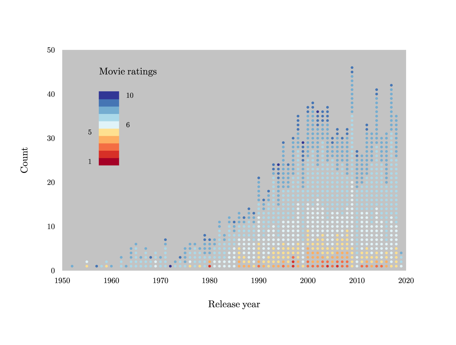
brewerusage.gle

! Example of dot chart with Brewer colors.
! Author: Francois Tonneau

! Plot idea from https://github.com/Pjarzabek/DotPlotPython

include brewer.gle

size 18.5 14

set font ss
set hei 0.4

! Prepare plot frame.

amove 2.5 3
begin graph
    size 14 9
    fullsize
    background "#c3c3c3"
    xaxis min 1950 max 2020 dticks 10
    yaxis min 0 max 50 dticks 10
    set just tc
    xlabels dist 0.3
    xtitle "Release year" dist 0.7
    set just cr
    ylabels dist 0.3
    ytitle "Count" dist 0.8
    ticks off
    side off
end graph

! Draw colored dots.

previous = -1
count = 0
fopen ratings.dat handle read
until feof(handle)
    fread handle year rating
    if year = previous then
        count = count + 1
    else
        count = 1
    end if
    amove xg(year) yg(count)
    ! Divergent palette with 10 colors: Rd = red, Yl = yellow, Bu = blue.
    hue$ = RdYlBuDiv10(rating)
    set color hue$ lwidth 0.001
    circle 0.05 fill hue$
    previous = year
next
fclose handle

! Add rating scale.

amove 4 2.3
begin origin

amove 0 5
for z = 1 to 10
    hue$ = RdYlBuDiv10(z)
    set color hue$ lwidth 0
    box 0.8 0.3 just bl fill hue$
    rmove 0 0.3
next z

amove 0 8.8
set color black hei 0.4 just cl
write "Movie ratings"

set hei 0.3 just cr
amove -0.3 5.15
write 1
amove -0.3 6.35
write 5
set just cl
amove 1.1 6.65
write 6
amove 1.1 7.85
write 10

end origin

colormap.gle

colormap.gle colormap.zip zip file contains all files for this figure.

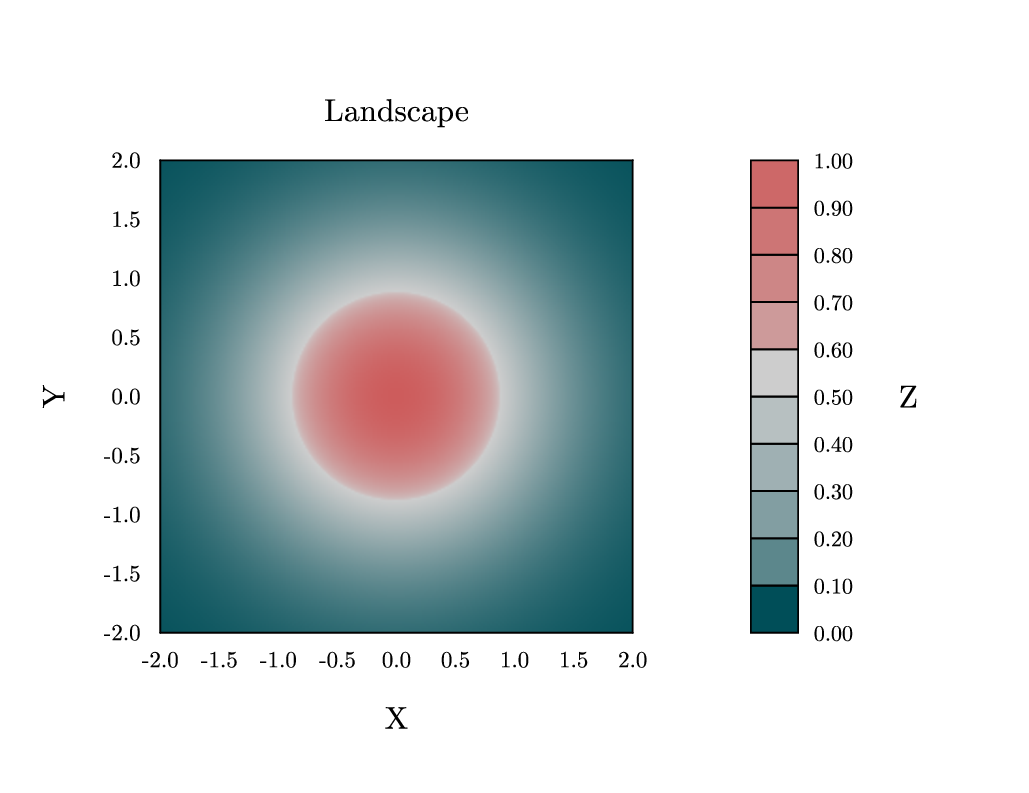
colormap.gle

! Example of a color map with a scale.
! Author: Francois Tonneau

! These are the number of steps we will require for a color gradient. Higher
! numbers result in a smoother gradient at the expense of processing time.
! Decrease x_steps and y_steps if the figure takes too long to appear.

x_steps = 250
y_steps = 250

size 13 10

set font ss

amove 2 2
begin graph
    size 6 6
    fullsize
    title "Landscape" hei 0.4 dist 0.5
    xaxis min -2 max 2
    yaxis min -2 max 2
    ticks off
    labels dist 0.25
    xtitle "X" hei 0.4 dist 0.5
    ytitle "Y" hei 0.4 dist 0.5

    ! When called from within a graph block, the 'colormap' command assumes a
    ! different, simpler syntax. The first argument is a subroutine that assigns
    ! a numeric value in the 0-1 range to (x, y) graph coordinates. The second
    ! and third arguments are the number of steps for x and y, respectively.
    ! The last argument (the one after the 'palette' keyword) is a custom
    ! color palette. *The first and last arguments should be non-quoted.*

    colormap z(x,y) x_steps y_steps palette glow
end graph

! Here is the subroutine we use to assign numeric values to (x, y) graph
! coordinates:

sub z x y
    local  sigma = 0.75
    local  value = exp(-(x^2 + y^2)/(2 * sigma^2))
    return value
end sub

! Our palette subroutine returns a nonlinear mixture (in standard RGB space) of
! three colors as a function of numeric input:

sub glow z
    local r_cool =   0; local g_cool =  78; local b_cool =  88
    local r_luke = 205; local g_luke = 205; local b_luke = 205
    local r_warm = 205; local g_warm =  92; local b_warm =  92
    if z < 0.50 then
        local w = sqrt(z/0.50)
        local r = w * r_luke + (1 - w) * r_cool
        local g = w * g_luke + (1 - w) * g_cool
        local b = w * b_luke + (1 - w) * b_cool
    end if
    if z >= 0.50 then
        local w = sqrt((z - 0.50)/0.50)
        local r = w * r_warm + (1 - w) * r_luke
        local g = w * g_warm + (1 - w) * g_luke
        local b = w * b_warm + (1 - w) * b_luke
    end if
    return rgb255(r, g, b)
end sub

set hei 0.28 just bl

! We add a custom color scale:

height = 2.0
width  = 0.6

for z = 0 to 0.9 step 0.1
    amove 9.5 height
    box width width fill glow(z)
    rmove 0.8 -0.1
    write format$(z, "fix 2")
    height = height + width
next z
rmove 0 width
write "1.00"

set hei 0.4 just cc
amove 11.5 5
write "Z"

! This script ends our tutorial. Although we have covered a lot of ground, feel
! free to consult the User Manual for the full details on these topics, as well
! as information on other GLE options and commands.

colormapcontour.gle

colormapcontour.gle colormapcontour.zip zip file contains all files for this figure.

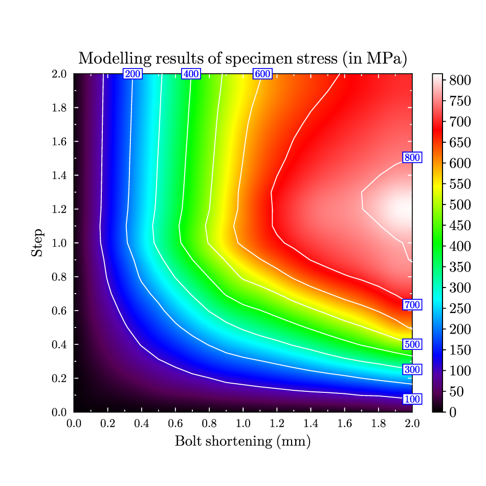
colormapcontour.gle

! Example of how to use color map and contour at the same time.
! Plot of modelling results coming from Abaqus.
! By Fabien Leonard.

size 12 12

set font texcmr

include "color.gle"
include "contour.gle"

! creates the z-value file to be used by the contour command
begin fitz
   data "Zstress.csv"
   x from 0 to 2 step 0.1
   y from 0 to 2 step 0.1
   ncontour 6
end fitz

begin contour    
   data "Zstress.z"
   values from 100 to 800 step 100
end contour

begin graph
   title "Modelling results of specimen stress (in MPa)"
   xtitle "Bolt shortening (mm)"
   ytitle "Step"
   xticks color white
   yticks color white
   colormap "Zstress.z" 500 500 color
   data "Zstress-cdata.dat"
   d1 line color white lwidth 0.02
end graph

amove xg(xgmax)+0.5 yg(ygmin)
color_range_vertical zmin 0 zmax 815 zstep 50 pixels 1500 format "fix 0"
contour_labels file "Zstress-clabels.dat" format "fix 0"

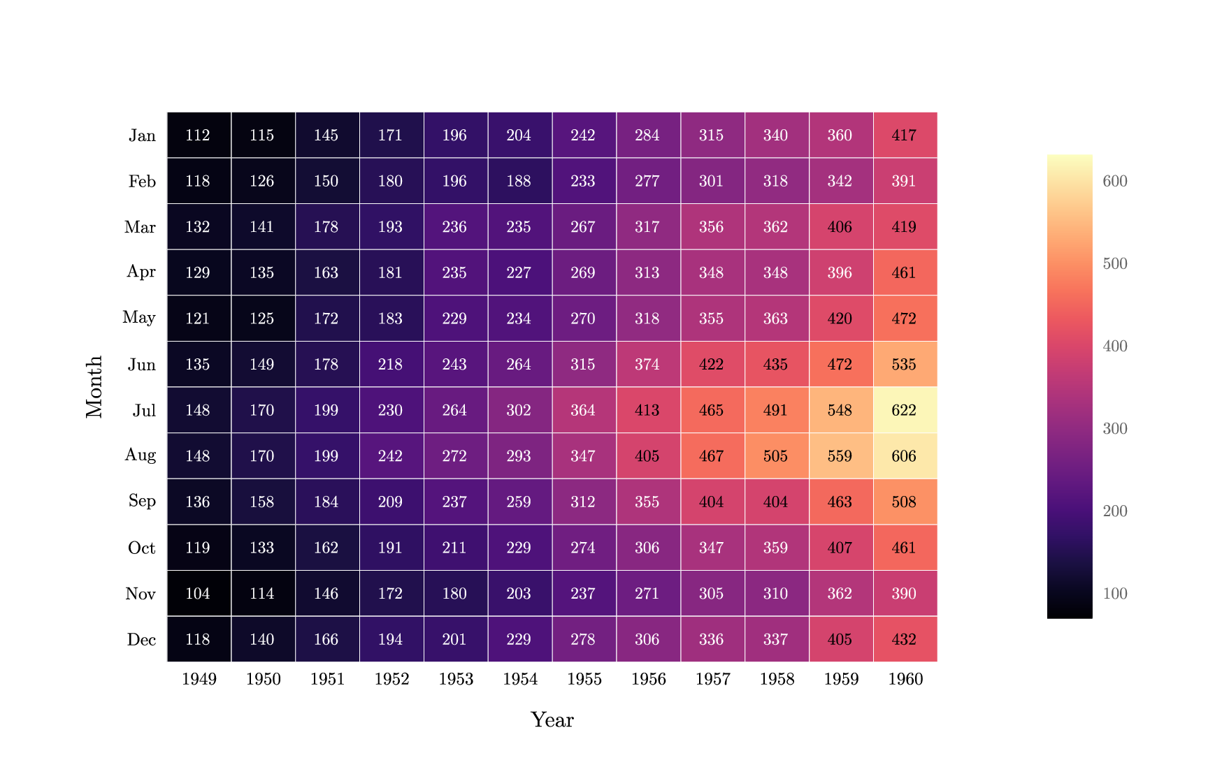
heatmap.gle

heatmap.gle heatmap.zip zip file contains all files for this figure.

heatmap.gle

! Example of heatmap with black/white numeric labels.
! Author: Francois Tonneau

size 22 14

set font ss hei 0.3

include palettes.gle

! Draw the frame around the map via a graph block.

amove 3 2
begin graph
    size 14 10
    fullsize
    xaxis min 0 max 12 ftick 0.5 dticks 1
    yaxis min 0 max 12 ftick 0.5 dticks 1
    xtitle Year adist 0.9
    ytitle Month adist 1.2
    side off
    ticks off
    xlabels off
    x2labels off
    ylabels off
    y2labels off
    labels hei 0.4
    data "heatmap.dat"
    xnames 1949 1950 1951 1952 1953 1954 1955 1956 1957 1958 1959 1960
    ynames Dec Nov Oct Sep Aug Jul Jun May Apr Mar Feb Jan
end graph

! Draw the map.

low = 100
high = 630

dx = xg(2) - xg(1)
dy = yg(2) - yg(1)

sub adjusted z
    return (z - low) / (high - low)
end sub

for col = 1 to ndatasets()
    n = ndata(d[col])
    for row = 1 to n
        z = datayvalue(d[col], row)
        amove xg(col - 1) yg(n - row)
        set color white lwidth 0.01
        box dx dy just bl fill magma(adjusted(z))
        rmove 0.33 0.32
        set color magma_text(adjusted(z))
        write z
    next row
next col

! Add a custom color ramp on the right.

low = 70        ! => stretch the ramp down for prettier looks
high = 630
dy = 0.015

amove 19 2.8
for z = low to high
    set color magma(adjusted(z)) lwidth 0
    box 0.8 dy just bl fill magma(adjusted(z))
    rmove 0 dy
next z
set color gray50 lwidth 0.03 just lc

amove 20 2.8+(30*dy)
for tick = 100 to 600 step 100
    write tick
    rmove 0 1.5
next tick

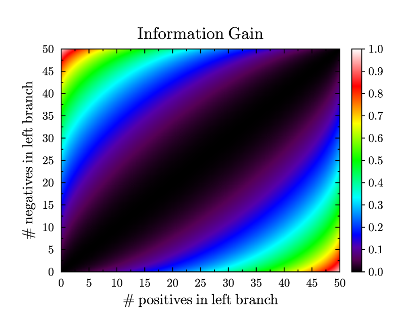
informationgain.gle

informationgain.gle informationgain.zip zip file contains all files for this figure.

informationgain.gle

size 10 8

include "color.gle"

set font texcmr

tpos = 50; tneg = 50
tot = tpos + tneg

sub entropy p
   if (p = 0) or (p = 1) then return 0
   else return -p*log(p)/log(2) - (1-p)*log(1-p)/log(2)
end sub

sub information_gain lpos lneg
   local rpos = tpos - lpos
   local rneg = tneg - lneg
   local ltot = lpos + lneg
   local rtot = rpos + rneg
   return entropy(tpos/tot) - &
      ltot/tot*entropy(sdiv(lpos,ltot)) - rtot/tot*entropy(sdiv(rpos,rtot))
end sub

begin graph
   xaxis min 0 max tpos
   yaxis min 0 max tneg
   title "Information Gain"
   xtitle "# positives in left branch"
   ytitle "# negatives in left branch"
   colormap information_gain(x,y) 250 250 color
end graph

set hei 0.29
amove xg(xgmax)+0.3 yg(ygmin)
color_range_vertical zmin 0 zmax 1 zstep 0.1 pixels 500 format "fix 1"

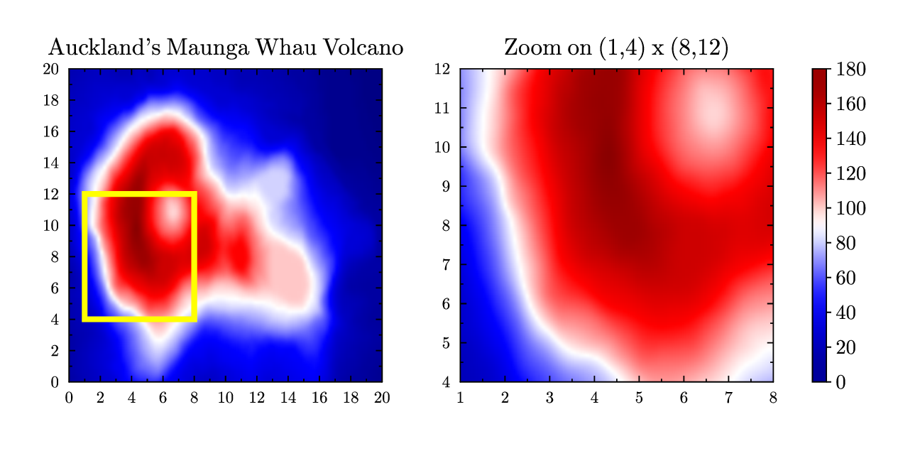
maungazoom.gle

maungazoom.gle maungazoom.zip zip file contains all files for this figure.

maungazoom.gle

size 16 8

include "color.gle"

! draw left graph
amove 0 0
begin graph
   size 8 8
   title "Auckland's Maunga Whau Volcano"
   colormap "volcano.z" 100 100 palette palette_blue_white_red
end graph

! define zoom rectangle on left graph
zx0 = 1; zy0 = 4
zx1 = 8; zy1 = 12

! draw zoom rectangle in yellow
gsave
set color yellow lwidth 0.1
amove xg(zx0) yg(zy0)
box xg(zx1)-xg(zx0) yg(zy1)-yg(zy0)
grestore

! draw right graph
amove 7 0
begin graph
   size 8 8
   title "Zoom on ("+num$(zx0)+","+num$(zy0)+") x ("+num$(zx1)+","+num$(zy1)+")"
   xaxis min zx0 max zx1
   yaxis min zy0 max zy1
   colormap "volcano.z" 100 100 palette palette_blue_white_red
end graph

! draw vertical color range
amove 14.5 yg(ygmin)
color_range_vertical zmin 0 zmax 180 zstep 20 palette palette_blue_white_red

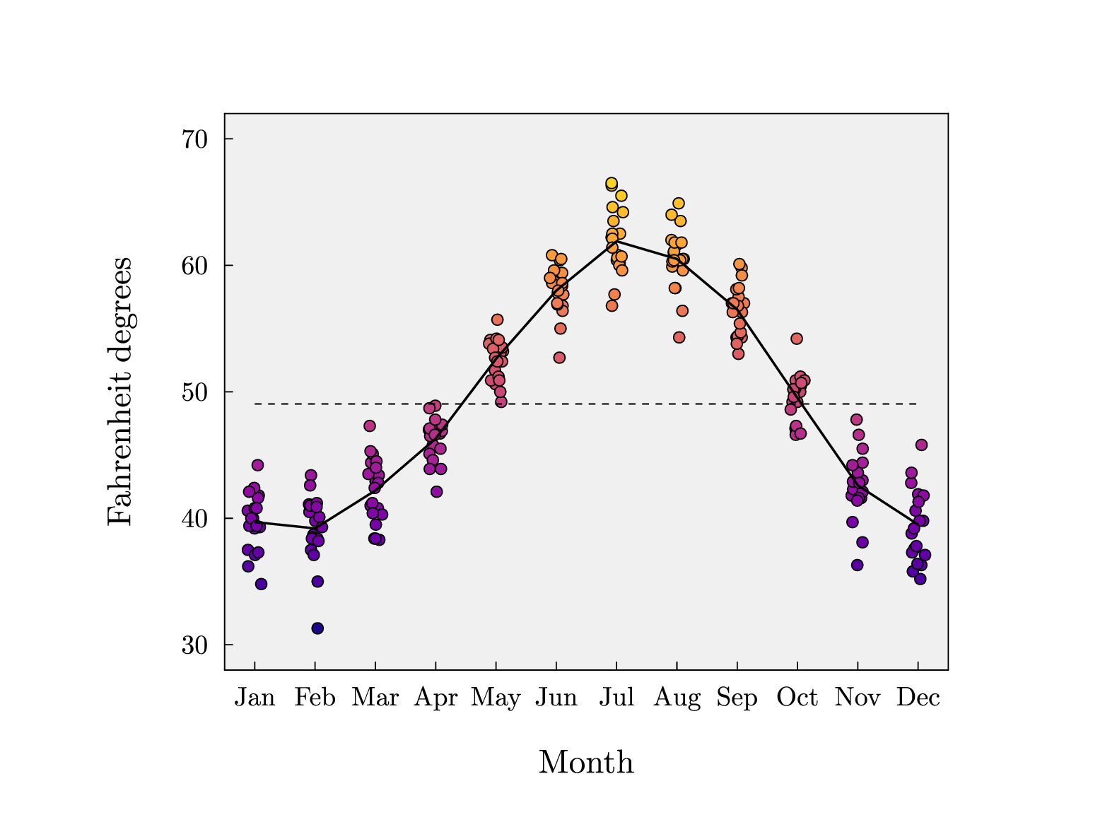
nottingham.gle

nottingham.gle nottingham.zip zip file contains all files for this figure.

nottingham.gle

! Example of scatter plot with colorized dots.
! Author: Francois Tonneau

size 20 15

include palettes.gle

amove 4 3

set font ss hei 0.6

! Plot data.

begin graph
    size 13 10
    fullsize
    background "#f0f0f0"
    xaxis min 0.5 max 12.5 ftick 1 dticks 1
    yaxis min 28 max 72 ftick 30 dticks 10
    ticks length 0.15
    x2ticks off
    y2ticks off
    subticks off
    xnames Jan Feb Mar Apr May Jun Jul Aug Sep Oct Nov Dec
    xtitle "Month" dist 0.7
    ytitle "Fahrenheit degrees" dist 0.8
    data "nottingham.dat"
    draw scatter                        ! plot monthly data with x jittering
    d21 line lwidth 0.04 color black    ! add line with 20-month averages
end graph

sub scatter
    local noise = 0.25
    local month, count, x, y, z, xp, yp
    for month = 1 to 20
        for count = 1 to ndata(d[month])
            x = dataxvalue(d[month], count)
            y = datayvalue(d[month], count)
            z = (y - 30) / (70 - 30)
            xp = xg(x) + rnd(noise) - noise/2
            yp = yg(y)
            amove xp yp
            set fill plasma(z)
            circle 0.10
        next count
    next month
end sub

! Add horizontal line with grand mean.

set lstyle 33
amove xg(1) yg(49.04)
aline xg(12) yg(49.04)

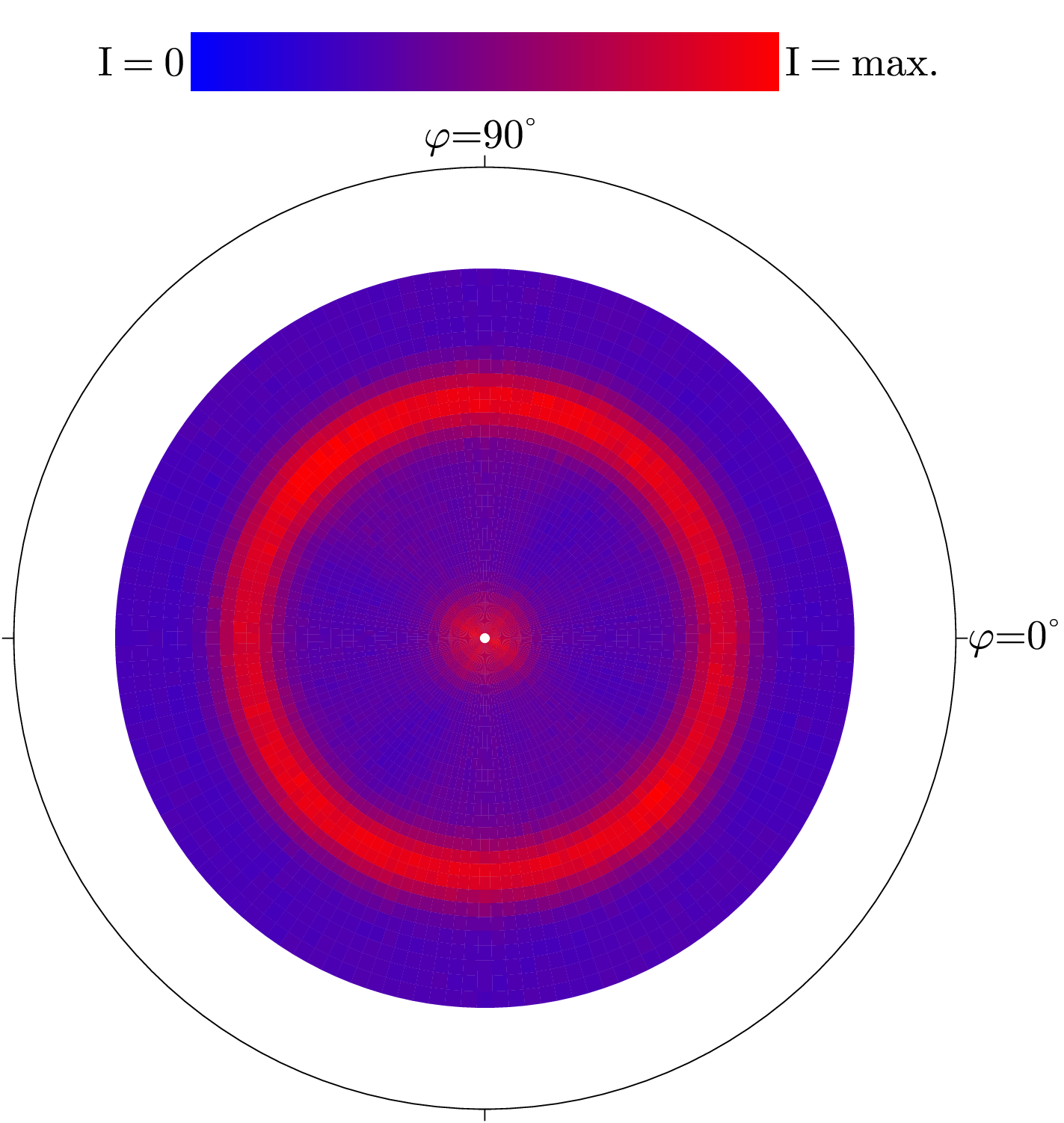
polenja.gle

polenja.gle polenja.zip zip file contains all files for this figure.

polenja.gle

size 18 19

include "color.gle"

set lwidth .02 hei .7 font texcmr
imax = 0; imaxc = 0

dpsi = 2.5; dphi = 2.5
! dpsi = stepwidth in psi direction, i.e. angle of latitude or elevation;
! dphi = stepwidth in phi direction, i.e. angle of longitude or azimuth.

file$ = "serguei2.nja"

! open result file with three rows: psi   phi   intensity
! first open to find overall maximum intensity = imax
! and maximum intensity at center = imaxc (i.e. for psi=0)

fopen file$ inchan read
until feof(inchan)
   fread inchan psi phi i
   if i>imax then
      imax = i
   end if
   if psi=0 then
      if i>imaxc then
         imaxc = i
      end if
   end if
next
fclose inchan

! now open result file for actual plotting
! colors are defined with rgb color scheme:
!     rgb(0,0,1) (i.e. blue) corresponds to i=0
!     rgb(1,0,0) (i.e. red) corresponds to i=max
fopen file$ inchan read
until feof(inchan)
   fread inchan psi phi i
   amove 8.2 8.2
   if psi=0 then
      circle dphi fill cvtrgb(imaxc/imax,0,1-imaxc/imax)
   else
      begin path fill cvtrgb(i/imax,0,1-i/imax)
         arc 8*sin(torad(psi+dpsi/2))/(1+cos(torad(psi+dpsi/2))) phi-dphi/2 phi+dphi/2
         narc 8*sin(torad(psi-dpsi/2))/(1+cos(torad(psi-dpsi/2))) phi+dphi/2 phi-dphi/2
      end path
   end if
next
fclose inchan

! labeling
circle 8
for c = 0 to 3
   begin rotate c*90
      rmove 8 0
      rline 0.2 0
   end rotate
next c

rmove 8.2 0
set just lc
write "\varphi =0\movexy{-.15}{0}\char{23}"
rmove -8.2 8.2
set just bc
write "\varphi =90\movexy{-.15}{0}\char{23}"

amove 8.2-5 17.5
begin name range
   colormap "x" 0 1 0 1 100 1 10 1 palette palette_blue_purple_red
end name

amove pointx(range.lc)-0.1 pointy(range.lc)
set just rc
write "I = 0"

amove pointx(range.rc)+0.1 pointy(range.rc)
set just lc
write "I = max."

ramps.gle

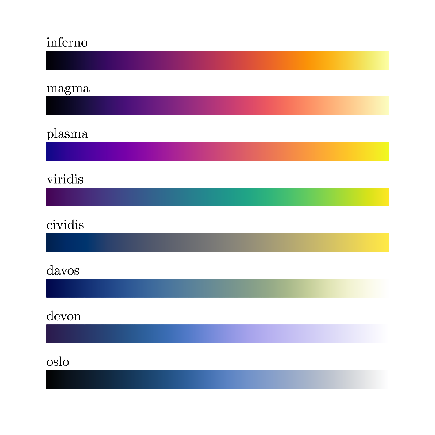
ramps.gle ramps.zip zip file contains all files for this figure.

ramps.gle

! Example with color ramps.
! Author: Francois Tonneau

size 19 19

set font ss hei 0.6

include palettes.gle

sub paintslice hue
    set color hue lwidth 0
    box 0.02 0.8 just bl fill hue
    rmove 0.02 0
end sub

amove 2 17
set color black
write "inferno"
rmove 0 -1
for z = 0 to 750
    paintslice inferno(z/750)
next z

amove 2 15
set color black
write "magma"
rmove 0 -1
for z = 0 to 750
    paintslice magma(z/750)
next z

amove 2 13
set color black
write "plasma"
rmove 0 -1
for z = 0 to 750
    paintslice plasma(z/750)
next z

amove 2 11
set color black
write "viridis"
rmove 0 -1
for z = 0 to 750
    paintslice viridis(z/750)
next z

amove 2 9
set color black
write "cividis"
rmove 0 -1
for z = 0 to 750
    paintslice cividis(z/750)
next z

amove 2 7
set color black
write "davos"
rmove 0 -1
for z = 0 to 750
    paintslice davos(z/750)
next z

amove 2 5
set color black
write "devon"
rmove 0 -1
for z = 0 to 750
    paintslice devon(z/750)
next z

amove 2 3
set color black
write "oslo"
rmove 0 -1
for z = 0 to 750
    paintslice oslo(z/750)
next z