Line Plots
Plots contianing lines generated from mathematical functions.
adjust.gle
 adjust.gle adjust.zip zip file contains all files for this figure.
adjust.gle
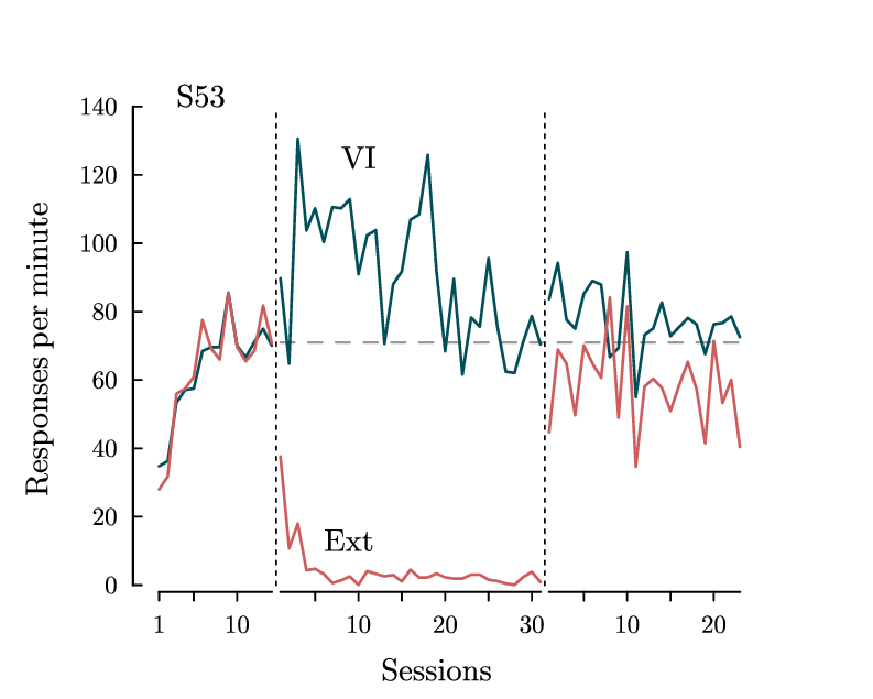
! Demo about plot adjustments.
! Author: Francois Tonneau

! In this script, data from different phases will be obtained from a tab-
! delimited file. By default, GLE does not connect data points across missing
! values. So, we have used the trick of inserting missing values ('*') into
! the data file to create visual breaks across phases.

size 10 8

set font ss cap round join round

begin graph

    xaxis min -2 max 68
    yaxis min -2 max 140 ftick 0 dticks 20

    ! We put custom tick labels ('xnames') at custom places along the x axis
    ! ('xplaces'):

    xplaces 1 10 24 34 44 55 65
    xnames  1 10 10 20 30 10 20

    x2axis   off
    y2axis   off
    side     off
    subticks off

    small = 0.1
    xticks length -small
    yticks length  small

    xtitle "Sessions" dist 0.3
    ytitle "Responses per minute" dist 0.3

    data "adjust.dat"

    ! Aside from named colors and the #RRGGBB notation, GLE lets us define hues
    ! with the rgb255() function. Each of its arguments is a number from 0 to
    ! 255, corresponding to the intensity of red, blue, and green.

    d1 line color rgb255(0,78,88)   lwidth 0.03
    d2 line color rgb255(205,92,92) lwidth 0.03

    ! We create a custom dataset to plot a horizontal line starting at x = 15:

    base_level = 71
    let d3 = base_level from 15 to 68

    ! GLE plots graphical elements through successive layers, the layer for
    ! data lines being layer #700. Creating a new layer with a number < 700
    ! forces the horizontal line to lie behind the data:

    begin layer 600
        d3 line color #999999 lstyle 44 lwidth 0.025
    end layer

end graph

set lwidth 0.025

! The xg() and yg() functions transform axis-relative coordinates (e.g., x = 1)
! into actual centimeters. These functions are very useful for positioning an
! object on the plot, but they cannot be called directly from a graph block --
! so we call them once the graph block is over. Here we use them to add line
! segments to the x axis:

amove xg(1)  yg(-2)
aline xg(14) yg(-2)

amove xg(15) yg(-2)
aline xg(45) yg(-2)

amove xg(46) yg(-2)
aline xg(68) yg(-2)

amove xg(-2) yg(0)
aline xg(-2) yg(140)

set lwidth 0.02

! We define a custom subroutine to add special ticks to the x axis:

sub add_tick place
    amove xg(place) yg(-2)
    rline 0 -small
end sub

add_tick 5

add_tick 19
add_tick 29
add_tick 39

add_tick 50
add_tick 60

! We also add vertical dashed lines to separate phases from one another:

set lstyle 12

amove xg(14.5) yg(0)
aline xg(14.5) yg(139)

amove xg(45.5) yg(0)
aline xg(45.5) yg(139)

! Finally, we add custom labels to the plot:

amove 2 yg(140)
write "S53"

amove xg(22) yg(122)
write "VI"

amove xg(20) yg(10)
write "Ext"

! Done. We have used layers as well as the xg() and yg() functions.
adphas.gle
 adphas.gle adphas.zip zip file contains all files for this figure.
adphas.gle
! Nice example by Axel Rohde
size 22 24
set font texcmr hei 0.55
x1 = -0.15; x2 = 0.6; xstep = 0.001
sub f x a
return pi+2*atn(a-sqrt(1-a^2)*tan(25*x*sqrt(1-a^2)/2))
end sub
sub do_label s$
gsave
set just cc
amove 0.75 yg(ygmax)+1
write s$; circle 0.4
grestore
end sub
amove 0 14
begin graph
size 25 9
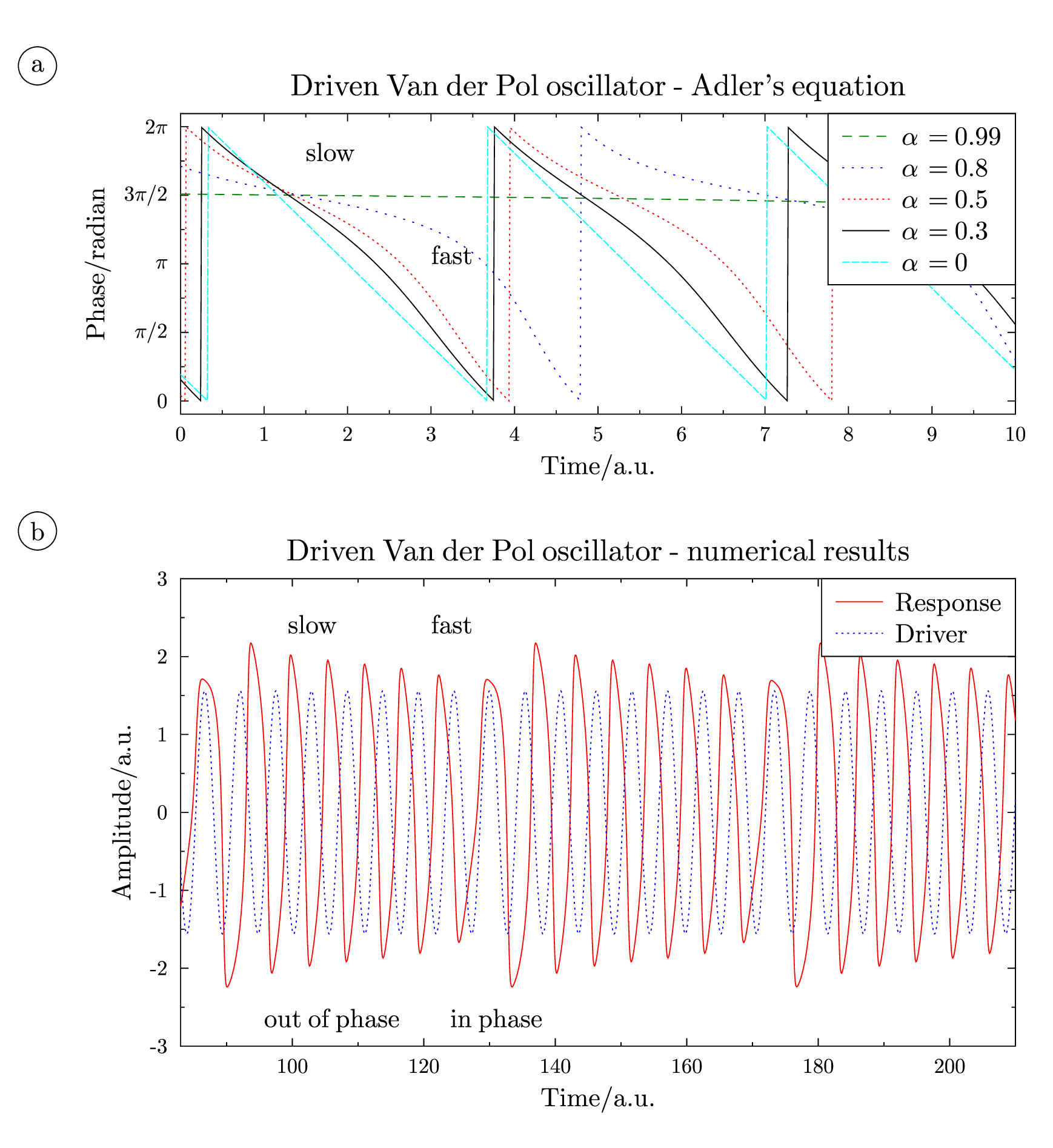
title "Driven Van der Pol oscillator - Adler's equation"
xtitle "Time/a.u."
ytitle "Phase/radian"
xaxis min 0 max 10
yaxis min -0.3 max 2*pi+0.3 ftick 0 dticks pi/2 format "pi"
key position tr
let d1 = f(x,0.99) from x1 to x2 step xstep
d1 line color green lstyle 9 xmin x1 xmax x2 key "\alpha\,= 0.99"
let d2 = f(x,0.8) from x1 to x2 step xstep
d2 line color blue lstyle 4 xmin x1 xmax x2 key "\alpha\,= 0.8"
let d3 = f(x,0.5) from x1 to x2 step xstep
d3 line color red lstyle 2 xmin x1 xmax x2 key "\alpha\,= 0.5"
let d4 = f(x,0.3) from x1 to x2 step xstep
d4 line color black lstyle 0 xmin x1 xmax x2 key "\alpha\,= 0.3"
let d5 = f(x,0) from x1 to x2 step xstep
d5 line color cyan lstyle 3 xmin x1 xmax x2 key "\alpha\,= 0"
end graph
do_label "a"
amove xg(3) yg(3.14)
write "fast"
amove xg(1.5) yg(5.5)
write "slow"
amove 0 0
begin graph
size 25 14
title "Driven Van der Pol oscillator - numerical results"
xtitle "Time/a.u."
ytitle "Amplitude/a.u."
xaxis min 83 max 210
yaxis min -3 max 3
data "adphas.dat"
let d4 = d3*1.2
key position tr
d1 line smooth lstyle 1 color red key "Response"
d4 line smooth lstyle 2 color blue key "Driver"
end graph
do_label "b"
amove 9 yg(2.3)
write "fast"
amove 6 yg(2.3)
write "slow"
amove 5.5 2.5
write "out of phase"
amove 9.4 2.5
write "in phase"
armand.gle
armand.gle
size 21.5 13.5
set font texcmr hei 0.5
a = 0.9; t = asin(a); s = sqrt(1-a^2)
amove 0.3 0.5
begin graph
size 12 8
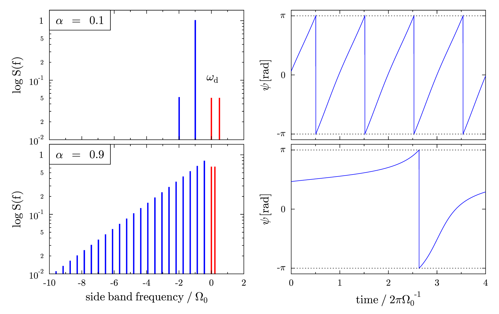
xtitle "side band frequency / \Omega_0"
ytitle "log S(f)"
xaxis min -10 max 2
yaxis min 10^-2 max 1.5 log
let d1 = tan(t/2) from 0 to s/2 step s
let d2 = (1-tan(t/2)^2)*(tan(t/2)^(-x-1)) from -46*s to -s step s
bar d1 width 0.05 color red fill red
bar d2 width 0.05 color blue fill blue
end graph
begin key
position tl
text "\alpha\:=\:0.9"
end key
a = 0.1; t = asin(a); s = sqrt(1-a^2)
amove 0.3 6.3
begin graph
size 12 8
xlabels off
ytitle "log S(f)"
xaxis min -10 max 2
yaxis min 10^-2 max 1.5 log
let d1 = tan(t/2) from 0 to s/2 step s
let d2 = (1-tan(t/2)^2)*(tan(t/2)^(-x-1)) from -100*s to -s step s
bar d1 width 0.05 color red fill red
bar d2 width 0.05 color blue fill blue
end graph
begin key
position tl
text "\alpha\:=\:0.1"
end key
amove xg(-0.3) yg(0.1)
write "\omega_d"
a = 0.9; omega = sqrt(1-a^2)
amove 10.75 0.5
begin graph
size 12 8
xtitle "time / 2\pi\Omega_0^{-1}"
ytitle "\psi\,\,[rad]"
xaxis min 0 max 4 dticks 1
yaxis min -0.3-pi max pi+0.3 ftick -pi dticks pi format "pi"
ysubticks off
let d1 = 2*atn(a+sqrt(1-a^2)*tan(0.5*sqrt(1-a^2)*omega*2*pi*x)) step 0.001
d1 line color blue
end graph
set lstyle 2
amove xg(0) yg(-pi)
aline xg(4) yg(-pi)
amove xg(0) yg(pi)
aline xg(4) yg(pi)
set lstyle 0
a = 0.1; omega = sqrt(1-a^2)
amove 10.75 6.3
begin graph
size 12 8
ytitle "\psi\,\,[rad]"
xaxis min 0 max 4 dticks 1
yaxis min -0.3-pi max pi+0.3 ftick -pi dticks pi format "pi"
ysubticks off
xlabels off
let d1 = 2*atn(a+sqrt(1-a^2)*tan(0.5*sqrt(1-a^2)*omega*2*pi*x)) step 0.001
d1 line color blue
end graph
set lstyle 2
amove xg(0) yg(-pi)
aline xg(4) yg(-pi)
amove xg(0) yg(pi)
aline xg(4) yg(pi)
set lstyle 0
bspline.gle
bspline.gle
size 10 8
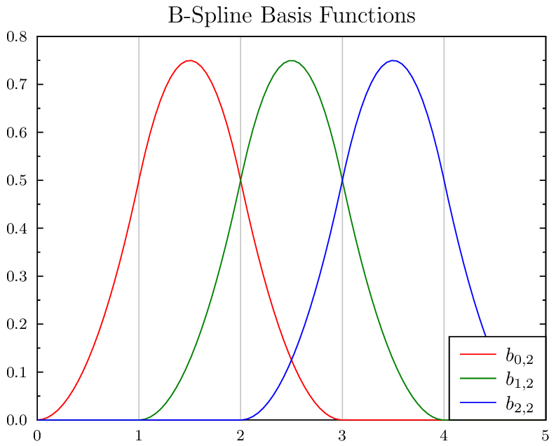
! http://en.wikipedia.org/wiki/B-spline
sub N j n x
if n = 0 then
if (x >= j) and (x < j+1) then return 1
else return 0
else
return (x-j)/n*N(j,n-1,x) + (j+n+1-x)/n*N(j+1,n-1,x)
end if
end sub
set texlabels 1
begin graph
scale auto
title "B-Spline Basis Functions"
xaxis min 0 max 5 dticks 1 grid
xticks color gray10
let d1 = N(0,2,x)
let d2 = N(1,2,x)
let d3 = N(2,2,x)
key pos br
d1 line color red key "$b_{0,2}$"
d2 line color green key "$b_{1,2}$"
d3 line color blue key "$b_{2,2}$"
end graph
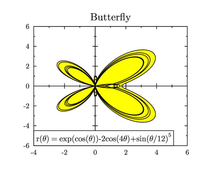
butterfly.gle
butterfly.gle
size 9 7

include "graphutil.gle"
include "polarplot.gle"

set font texcmr
begin graph
   math
   title "Butterfly"
   xaxis min -4 max 6 dticks 2
   yaxis min -6 max 6 dticks 2
   labels off
   x0labels on
   y0labels on
   x2axis on
   y2axis on
   draw polar "exp(cos(t))-2*cos(4*t)+sin(t/12)^5" 0 12*pi fill yellow
end graph

set color black hei 0.33 just bl
graph_textbox label "r(\theta) = exp(cos(\theta))-2cos(4\theta)+sin(\theta/12)^5"
compactkey.gle

compactkey.gle
size 12 9

set font texcmr
begin graph
   scale auto
   title "``Compact'' key mode"
   yaxis dticks 0.5
   xaxis min 0 max 2*pi dticks pi/4 format "pi"
   let d1 = sin(x)
   let d2 = cos(x)
   key pos bl compact offset 0.2 0.2
   d1 line color red  marker triangle mdist 1 key "Sine"
   d2 line color blue marker circle   mdist 1 key "Cosine"
end graph
diffeq.gle
diffeq.gle
size 10 8
include "graphutil.gle"
sub plotone x0 y0 cnt
amove xg(x0) yg(y0)
for i = 0 to cnt
x0 = x0+y0*dt
y0 = y0+(y0*(1-x0^2)-x0)*dt
if (x0<-3) or (x0>3) or (y0<-3) or (y0>3) then
i = cnt
end if
aline xg(x0) yg(y0)
next i
end sub
sub plotall
dt = 0.05
set color gray40
graph_line 0 -3 0 3
graph_line -3 0 3 0
set color rgb255(38,38,134)
plotone -0.25 0 250
plotone -0.1 0 250
plotone 0.1 0 250
plotone 0.25 0 250
for j=0 to 3
plotone -3 j 100
plotone 3 -j 100
next j
for j=-3 to 3 step 0.25
plotone -j 3 100
plotone j -3 100
next j
end sub
set texlabels 1
begin graph
scale auto
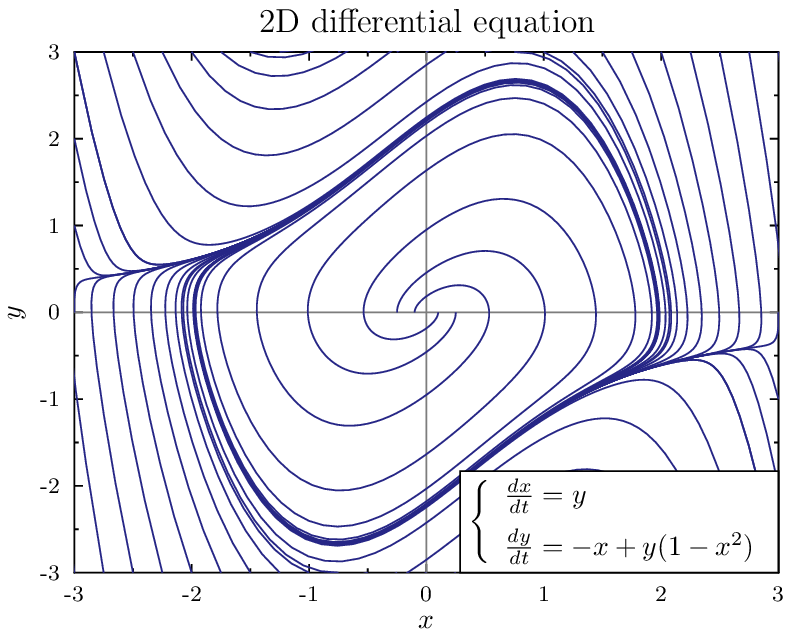
title "2D differential equation"
xtitle "$x$"
ytitle "$y$"
xaxis min -3 max +3
yaxis min -3 max +3
draw plotall
end graph
begin object key
begin box add 0.1 fill white
begin tex
$\left\{ \begin{array}{l}
\frac{dx}{dt}=y\vspace{0.2cm}\\
\frac{dy}{dt}=-x+y(1-x^2)
\end{array} \right.$
end tex
end box
end object
amove xg(xgmax) yg(ygmin)
draw key.br
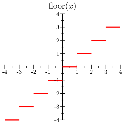
discontinuity.gle
discontinuity.gle
size 6 6

set texlabels 1
xmin = -4; xmax = 4

sub floor x
   if x>=0 then
       return int(x)
   else if x=int(x) then
       return int(x)
   else
       return int(x)-1
   end if
end sub

begin graph
   math
   scale auto
   xaxis min xmin max xmax
   labels dist 0.15
   xaxis format "fix 0"
   yaxis format "fix 0"
   x2axis off
   y2axis off
   title "$\mathrm{floor}(x)$"
   discontinuity threshold 5
   let d1 = floor(x) step 0.1
   d1 line color red lwidth 0.05
end graph
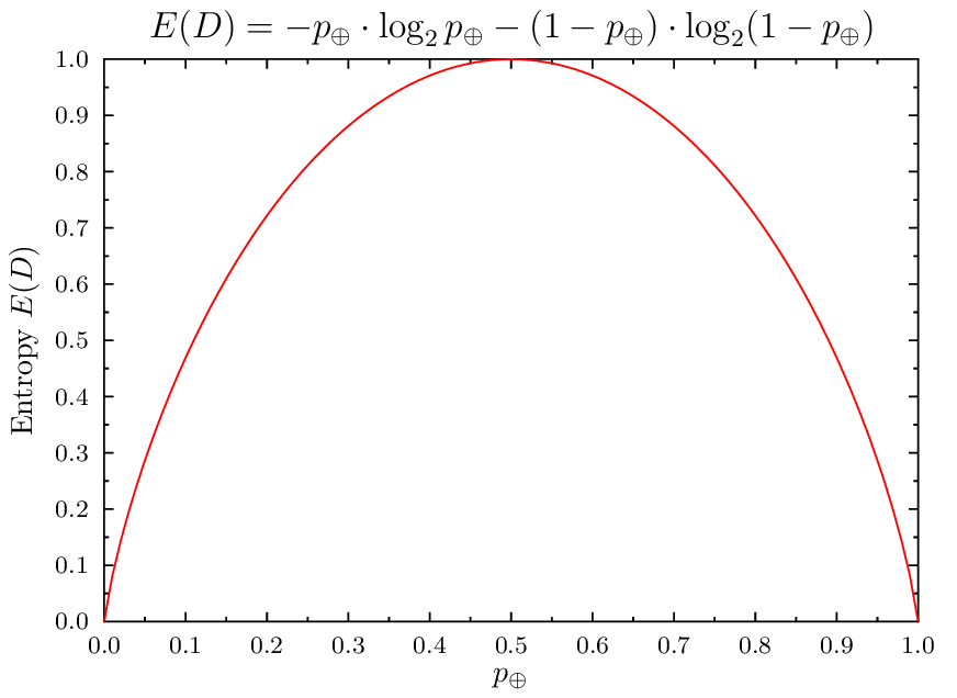
entropy.gle
entropy.gle
size 11 8

sub entropy x
   return (-x)*log(x)/log(2)-(1-x)*log(1-x)/log(2)
end sub

set texlabels 1
begin graph
   scale  auto
   title  "$E(D) = -p_\oplus \cdot \log_2 p_\oplus - (1-p_\oplus) \cdot \log_2 (1-p_\oplus)$"
   xtitle "$p_\oplus$"
   ytitle "Entropy $E(D)$"
   let d1 = entropy(x) from 0 to 1
   d1 line color red
end graph
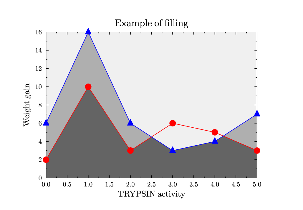
fill.gle
 fill.gle fill.zip zip file contains all files for this figure.
fill.gle
size 13 9

set font texcmr
begin graph
   title  "Example of filling"
   xtitle "TRYPSIN activity"
   ytitle "Weight gain"
   data   "test.dat"
   d1 line marker fcircle   color red
   d2 line marker ftriangle color blue
   fill x1,d1 color gray50
   fill d1,d2 color gray20
   fill d2,x2 color gray5
end graph
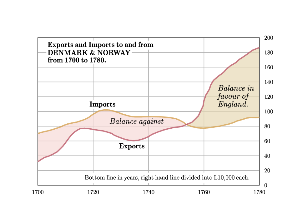
fill-ft.gle
 fill-ft.gle fill-ft.zip zip file contains all files for this figure.
fill-ft.gle
! Example of curve filling with semi-transparency.
! Author: Francois Tonneau

! *Because this figure involves semi-transparent elements, it must be compiled
! with the -cairo option:*

! gle -cairo -d pdf fill.gle

! Not including this option will result in compilation failure.

size 12 9

set font texcmr

amove 1.5 1.5
begin graph
    size 9 6
    fullsize
    xaxis min 1700 max 1780 dticks 20 hei 0.3 grid color gray20
    yaxis min 0 max 200 dticks 20 hei 0.3 grid color gray20
    side color gray70
    labels color black dist 0.2
    ylabels off
    y2labels on

    data "fill-ft.dat" d1=c1,c2 d2=c3,c4

    ! We plot our data sets with Savitsky-Golay smoothed curves ('svg_smooth')
    ! and semi-transparent hues. The rgba255() function accepts four channel
    ! values in the 0-255 range: red, green, blue, and alpha/transparency.

    d1 svg_smooth line color rgba255(213,162,83,200) lwidth 0.05
    d2 svg_smooth line color rgba255(187,89,105,200) lwidth 0.05

    ! GLE can fill areas between an axis and a dataset or between different
    ! datasets. Also, filling can be clipped between minimal and maximal values.
    ! Here we add two semi-transparent fills to the plot, one to the left of
    ! x = 1754 and the other to the right; 1754 is where the curves of the
    ! d1 and d2 datasets cross.

    light$  = rgba255(247, 218, 215, 180)
    medium$ = rgba255(231, 217, 181, 180)

    fill d1,d2 color light$  xmin 1700 xmax 1754
    fill d1,d2 color medium$ xmin 1754 xmax 1780
end graph

! We add labels to the plot:

set font texcmti hei 0.325

amove 4.4 4
write "Balance against"

! Because the 'write' command cannot deal with multi-line labels, for our next
! label we employ a 'begin text ... end text' block:

amove 8.80 5.35
begin text
    Balance in
    favour of
    England.
end text

set font texcmb hei 0.3

! All the other labels are inserted in 'begin box ... end box' blocks to give
! the labels a rectangular white background. The 'add' option specifies the
! amount of padding between the text and the border of the box; 'nobox'
! means that the border will not be actually drawn:

amove 3.6 4.7
begin box add 0.05 nobox fill white
    write "Imports"
end box

amove 4.8 3.0
begin box add 0.05 nobox fill white
    write "Exports"
end box

set font texcmb hei 0.3 just lc

amove 1.9 7.2
begin box add 0.05 nobox fill white
    write "Exports and Imports to and from"
end box
rmove 0 -0.3
begin box add 0.05 nobox fill white
    write "DENMARK & NORWAY"
end box
rmove 0 -0.3
begin box add 0.05 nobox fill white
    write "from 1700 to 1780."
end box

set font texcmr hei 0.25 just lc

amove 3.4 1.8
begin box add 0.10 nobox fill white
    write "Bottom line in years, right hand line divided into L10,000 each."
end box

! Done. We have learned about curve filling, rgba255() transparency, 'begin
! text ... end text' blocks, and 'begin box ... end box' blocks.
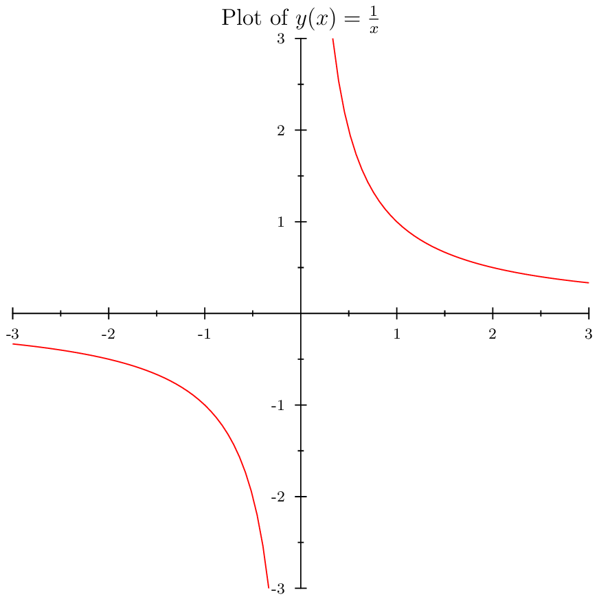
hyperbola.gle
hyperbola.gle
size 11 11

set texlabels 1
begin graph
   math
   scale auto
   title "Plot of $y(x) = \frac{1}{x}$"
   yaxis min -3 max 3
   let d1 = 1/x from -3 to 3
   d1 line color red
end graph
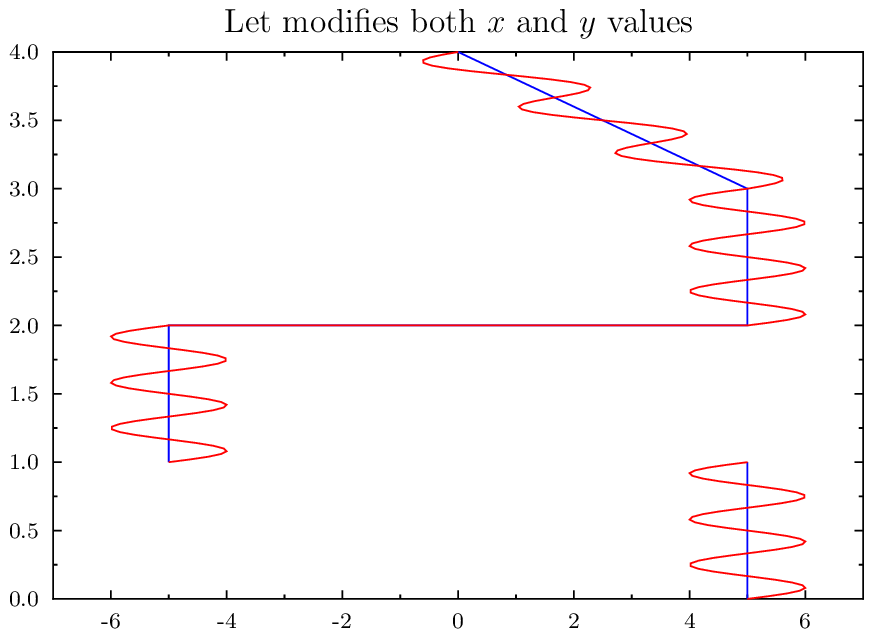
let-multi-dim.gle
 let-multi-dim.gle let-multi-dim.zip zip file contains all files for this figure.
let-multi-dim.gle
size 11 8

set texlabels 1
begin graph
   scale auto
   title "Let modifies both $x$ and $y$ values"
   xaxis min -7 max 7
   yaxis min 0 max 4
   data "let-multi-dim.csv"
   let d2 = d1, x
   let d3 = d1+sin(6*pi*x), x from 0 step 0.02
   d2 line color blue
   d3 line color red
end graph
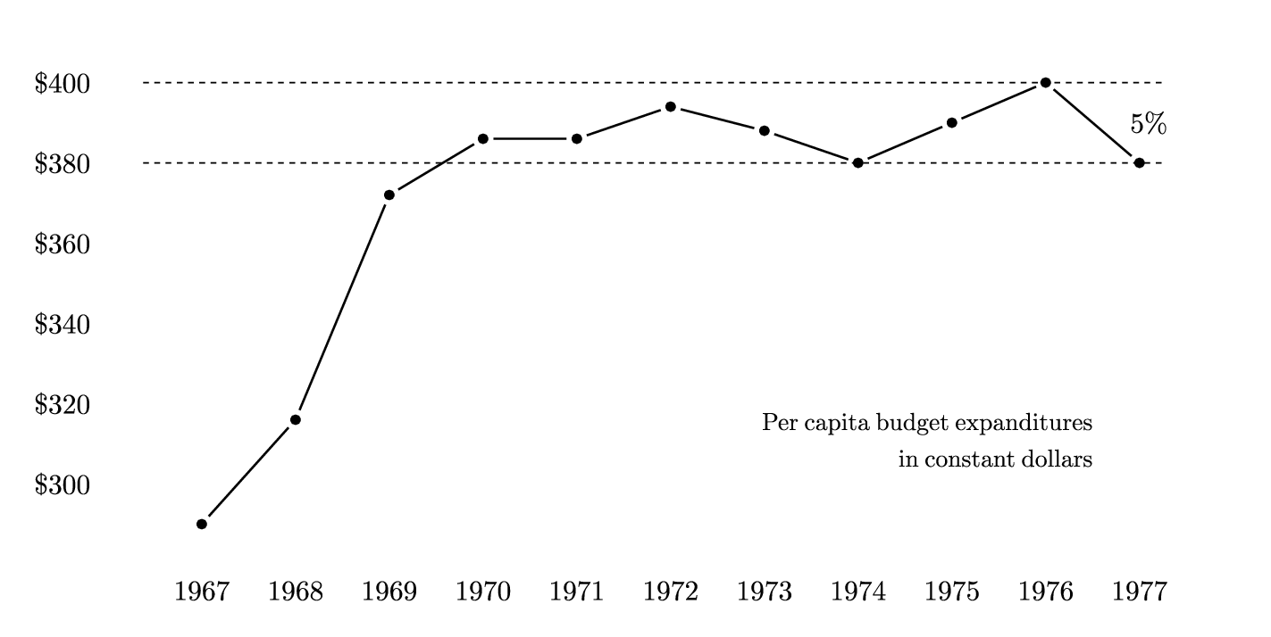
line.gle
 line.gle line.zip zip file contains all files for this figure.
line.gle
! Example of line plot.
! Author: Francois Tonneau

include openline.gle

size 18 9

set lwidth 0.03

amove 1.5 1
begin graph
    size 16 8
    fullsize
    xaxis min 1966 max 1978 ftick 1967 dticks 1 nolast
    yaxis min 0 max 7 ftick 1
    side  off
    ticks off
    labels color black font rm hei 0.5
    ynames  $300 $320 $340 $360 $380 $400
    data "line.dat"
    d1 marker dot msize 0.35
    draw openline d1 0.3
end graph

set lstyle 22 lwidth 0.02
amove 2 yg(5)
rline 14.5 0
amove 2 yg(6)
rline 14.5 0

set font rm hei 0.4 just cc
amove xg(1977.1) yg(5.5)
write "5%"

set hei 0.35 just cr
amove 15.5 3
write "Per capita budget expanditures"
amove xend() yend()
rmove 0 -0.4
write "in constant dollars"
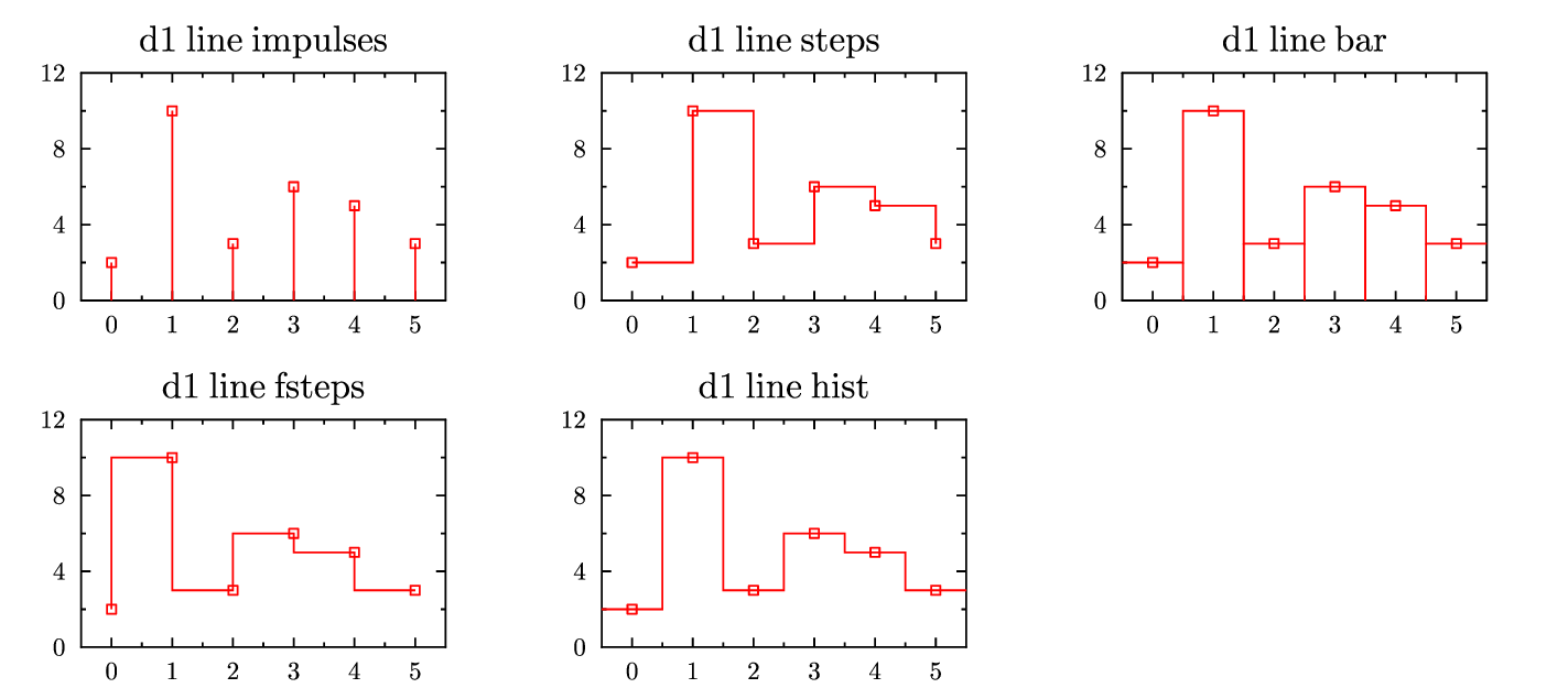
linemode.gle
 linemode.gle linemode.zip zip file contains all files for this figure.
linemode.gle
size 18 8

set font texcmr
sub linemode xp yp type$
   amove xp*6 yp*4
   begin graph
      size 6 3.75
      data  "test.dat"
      title "d1 line "+type$
      yaxis min 0 max 12 dticks 4
      xaxis min -0.5 max 5.5
      d1 line \expr{type$}
      d1 marker square msize 0.15 color red
   end graph
end sub

linemode 0 1 "impulses"
linemode 1 1 "steps"
linemode 0 0 "fsteps"
linemode 1 0 "hist"
linemode 2 1 "bar"
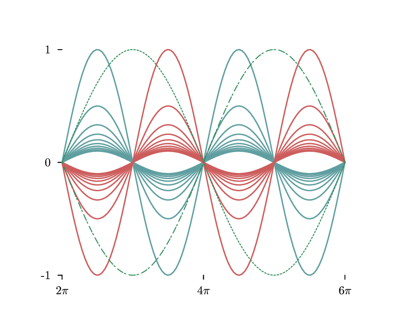
lines.gle
lines.gle
! Demo about line styles.
! Author: Francois Tonneau

size 10 8

set font ss

! We set line termination ('cap') to 'round' (other possible values are 'butt'
! and 'square'):

set cap round

begin graph

    ! In defining axis limits we use 'pi' (= 3.14...), which is a pre-declared
    ! variable in GLE. As usual, arithmetic expressions may not contain spaces:

    xaxis min 2*pi max 6*pi dticks 2*pi
    yaxis min -1 max 1 dticks 1

    ! We remove the axes and parts of axes (such as their spine or 'side') we
    ! don't want:

    x2axis   off
    y2axis   off
    xside    off
    yside    off
    subticks off

    ! We now define custom names for the x-axis ticks with the 'xnames' command.
    ! Quotes are not needed, any sequence of non-blank chars will be interpreted
    ! as a name. Each '\pi' expression (notice the backslash) will render as the
    ! Greek symbol, pi:

    xnames 2\pi 4\pi 6\pi

    ! A negative tick length makes the ticks face outward:

    ticks length -0.1

    ! In GLE, datasets d1, d2, ... can also be referred to as d[1], d[2], etc.
    ! The d[i] bracket notation for datasets is useful in scripts, especially
    ! when combined with loops, because the term inside [] can be any integer
    ! variable or expression. In this script we will use two 'for ... next'
    ! loops to define and plot 20 datasets in succession.

    ! First, we use a loop with the 'num' index to define and plot 10 blue
    ! curves. Because 'sin(x)' is divided by 'amplitude', the curves being
    ! drawn are progressively flatter:

    for num = 1 to 10
        amplitude  = num
        let d[num] = sin(x)/amplitude
        d[num] line color cadetblue lwidth 0.03
    next num

    ! We then use another loop to define and plot 10 red curves. As in the
    ! previous loop, the curves being drawn are progressively flatter:

    for num = 11 to 20
        amplitude  = num-10
        let d[num] = -sin(x)/amplitude
        d[num] line color indianred lwidth 0.03
    next num

    ! We finish the plot by adding two dashed lines. In GLE, a dash pattern is
    ! specified as a series of digits, each digit defining the length of a dash
    ! or a space (by default the pattern is '1', meaning a solid line):

    let d22 = sin(x/2)
    d22 line color seagreen lstyle 1241
    let d23 = -sin(x/2)
    d23 line color seagreen lstyle 11

end graph

! Done. We have learned about the d[...] bracket notation, 'for ... next' loops,
! and dashes. We have used 23 datasets -- in GLE 4.2 one can use up to 1000.
lnx.gle

lnx.gle
size 9 7

include "shape.gle"
include "graphutil.gle"

a = 4

! draw graph
set texlabels 1
begin graph
   scale auto
   title "Natural Logarithm"
   xtitle "$x$"
   ytitle "$y$"
   xaxis min 0 max a+1
   yaxis min 0 max 1.2
   let d1 = 1/x
   let d2 = 1/x from 1 to a
   d1 line color red
   fill x1,d2 color moccasin
end graph

! draw vertical red lines
set color red
graph_line 1 0 1 1
graph_line a 0 a 1/a
set color black

! draw integral equation
set just cc
amove xg(2.5) yg(0.18)
tex "$\displaystyle\log a = \int_{1}^{a}{\textstyle \frac{1}{x}\,dx}$"

! define subroutine to add labels to graph
sub label_by_dist_angle xp yp label$ dist angle
   default dist 0.75
   default angle 90
   amove xg(xp) yg(yp); pmove dist angle
   set just bc; tex label$
   amove xg(xp) yg(yp); pmove dist-0.1 angle
   aline xg(xp) yg(yp) arrow end
end sub

! draw "a" and "1/x"
label_by_dist_angle a    1/a    "$a$"
label_by_dist_angle 1.75 1/1.75 "$y = \frac{1}{x}$" angle 40
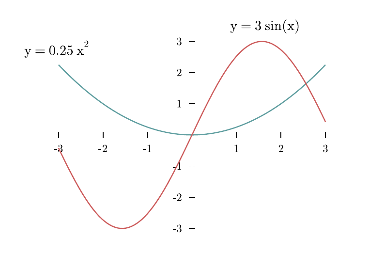
math_mode_plot.gle
math_mode_plot.gle
! Demo about plotting functions.
! Author: Francois Tonneau

size 10 7

set font ss

! We use a 'begin graph ... end graph' block to plot two simple mathematical
! functions.

begin graph

    ! The effect of the 'math' command is that axes cross at point (0, 0) and
    ! that axis ticks extend on both sides of the axis.

    math

    ! Regardless of the 'math' command, there are many ways to customize axes
    ! in GLE. Here we specify the minimum, maximum, and numerical distance
    ! between ticks for the x axis. We also specify tick length and remove
    ! subticks from all axes. Anything about axes that is not customized
    ! assumes default values.

    xaxis min -3 max 3 dticks 1
    ticks length 0.08
    subticks off

    ! The 'let' command allows us to define datasets as mathematical functions
    ! (i.e., expressions of x) instead of values loaded from a data file. The
    ! defining expressions may include parentheses and usual math operators,
    ! but must be written without spaces.

    let d1 = (1/4)*(x^2)
    let d2 = 3*sin(x)

    ! Now we can plot our previously defined datasets:

    d1 line color cadetblue lwidth 0.03
    d2 line color indianred lwidth 0.03

end graph

! We add descriptions of our functions to the plot. GLE has a variety of text
! formatting operators, such as the '^{...}' operator to produce superscript:

amove 0.6 5.6
write "y = 0.25 x^{2}"

amove 6 6.25
write "y = 3 sin(x)"

! Done. We have learned about function plotting and about the math mode of axis
! customization.
quantilescale.gle
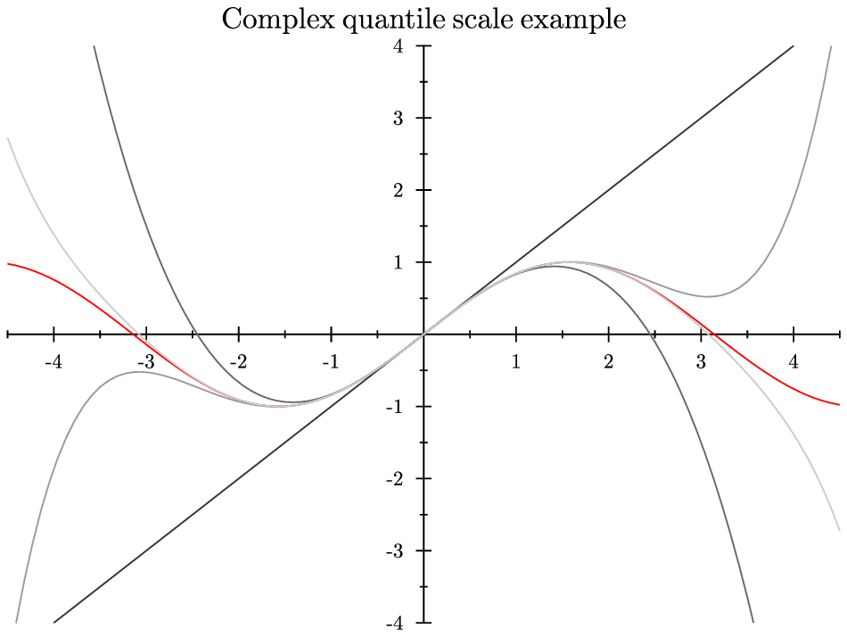
quantilescale.gle
size 12 9

set font texcmr
begin graph
   math
   scale auto
   title "Complex quantile scale example"
   xaxis min -4.5 max 4.5
   yaxis scale quantile
   let d1 = sin(x)
   d1 line color red
   let d2 = x
   d2 line color 0.2
   let d3 = x-x^3/6
   d3 line color 0.4
   let d4 = x-x^3/6+x^5/120
   d4 line color 0.6
   let d5 = x-x^3/6+x^5/120-x^7/5040
   d5 line color 0.8
end graph
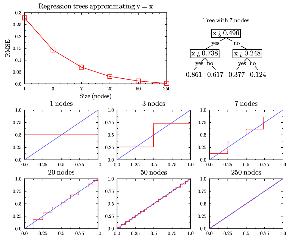
rt-y-is-x.gle
 rt-y-is-x.gle rt-y-is-x.zip zip file contains all files for this figure.
rt-y-is-x.gle
size 12 10

set font texcmr hei 0.26
include "simpletree.gle"

! Draw the main graph (RMSE versus number of nodes in regression tree)
amove 1 6.5
begin graph
   size 6 3
   fullsize
   title  "Regression trees approximating y = x"
   data   "rt-y-is-x-labels.dat"
   xtitle "Size (nodes)"
   ytitle "RMSE"
   xplaces 1 2 3 4  5  6
   xnames  1 3 7 20 50 250
   xaxis min 1 max 6
   yaxis max 0.3
   d3 line color red marker square
end graph

! Draw an example regression tree with 7 nodes
! x > 0.496
! +--yes: x > 0.738
! |       +--yes: 0.861
! |       +--no:  0.617
! +--no:  x > 0.248
!         +--yes: 0.377
!         +--no:  0.124

gsave
set just bc
amove (xg(6)+pagewidth())/2 pageheight()-0.9
write "Tree with 7 nodes"
binrootnode xpos() ypos()-0.3 "x > 0.496" "yes" "no" 1
  binnode "r1" "x > 0.738" "yes" "no" 0.5
    leaf "r11" "0.861"
    leaf "r12" "0.617"
  binnode "r2" "x > 0.248" "yes" "no" 0.5
    leaf "r21" "0.377"
    leaf "r22" "0.124"
grestore

sub bluediagonal
   set color rgb255(100,100,255)
   amove xg(0) yg(0); aline xg(1) yg(1)
   set color black
end sub

! Draw one of the small graphs (make sure the red goes over the blue)
sub plot x y n nodes
   amove x*3.9+1 y*2.9+0.4
   begin graph
      size 3.1 2.1
      fullsize
      data "rt-y-is-x.dat"
      d[n] line color red
      title "\expr{nodes} nodes"
      xaxis min 0 max 1 dticks 0.25
      yaxis min 0 max 1 dticks 0.25
      draw bluediagonal
   end graph
end sub

! Loop to draw the 6 small graphs
number = 1
fopen "rt-y-is-x-labels.dat" f1 read
for y = 1 to 0 step -1
   for x = 0 to 2
      fread f1 idx nodes mse rmse
      plot x y number nodes
      number = number+1
   next x
next y
fclose f1
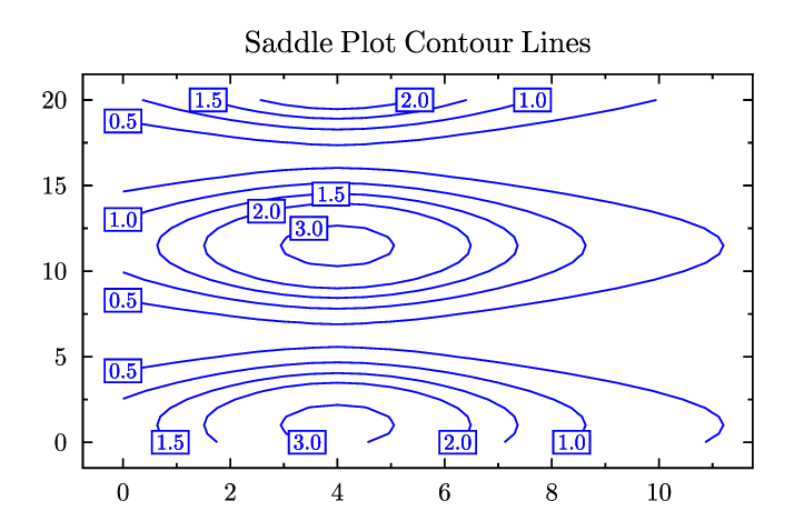
saddle-contour.gle
 saddle-contour.gle saddle-contour.zip zip file contains all files for this figure.
saddle-contour.gle
size 9 6

include "contour.gle"

set font texcmr

begin letz
   data "saddle.z"
   z = 3/2*(cos(3/5*(y-1))+5/4)/(1+(((x-4)/3)^2))
   x from 0 to 20 step 0.5
   y from 0 to 20 step 0.5
end letz

begin contour
   data "saddle.z"
   values 0.5 1 1.5 2 3
end contour

begin graph
   scale 0.85 0.75 center
   title "Saddle Plot Contour Lines" hei 0.35
   data "saddle-cdata.dat"
   xaxis min -0.75 max 11.75
   yaxis min -1.5 max 21.5
   d1 line color blue
end graph

contour_labels "saddle-clabels.dat" "fix 1"
semitrans.gle
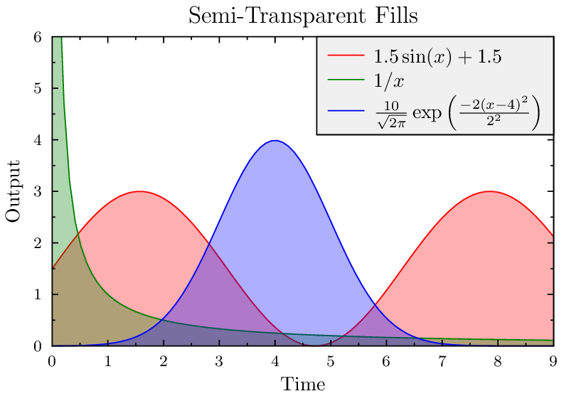
semitrans.gle
size 10 7
set font texcmss
set texlabels 1

begin graph
   scale auto
   title  "Semi-Transparent Fills"
   xtitle "Time"
   ytitle "Output"
   xaxis min 0 max 9
   yaxis min 0 max 6 dticks 1
   let d1 = sin(x)*1.5+1.5 from 0 to 10
   let d2 = 1/x from 0.01 to 10
   let d3 = 10*(1/sqrt(2*pi))*exp(-2*(sqr(x-4)/sqr(2))) from 0 to 10
   key background gray5
   begin layer 300
      fill x1,d1 color rgba255(255,0,0,80)
      d1 line color red key "$1.5\sin(x)+1.5$"
   end layer
   begin layer 301
      fill x1,d2 color rgba255(0,128,0,80)
      d2 line color green key "$1/x$"
   end layer
   begin layer 302
      fill x1,d3 color rgba255(0,0,255,80)
      d3 line color blue key "$\frac{10}{\sqrt{2\pi}}\exp\left(\frac{-2(x-4)^2}{2^2}\right)$"
   end layer
end graph
shadow.gle
shadow.gle
size 12 8
include "graphutil.gle"
set font texcmr
amove 0 0.3
begin graph
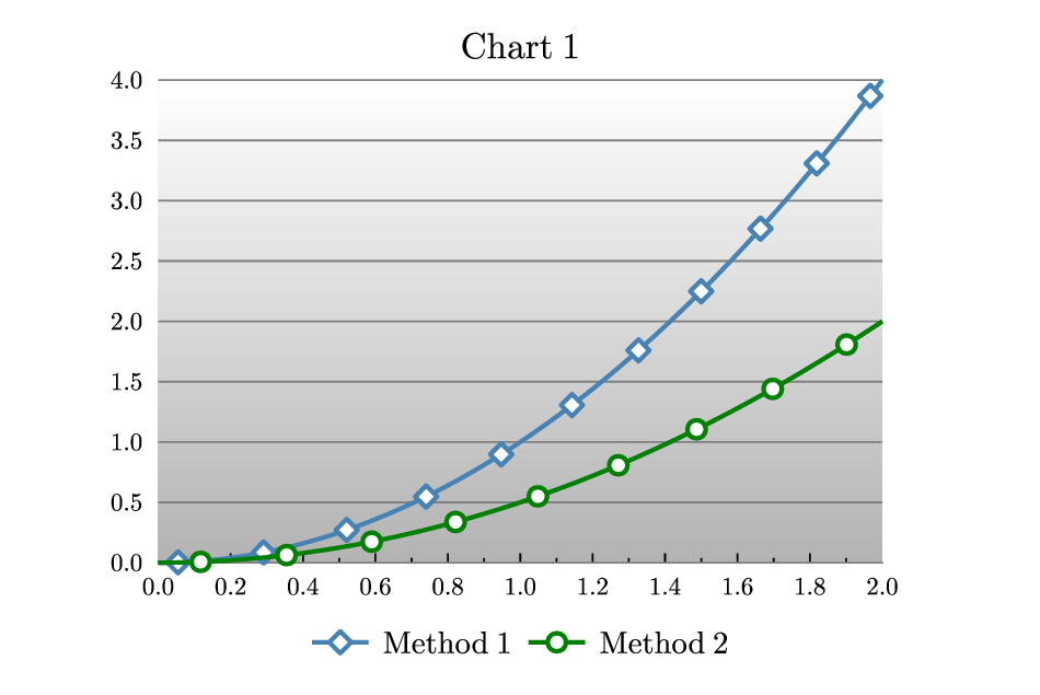
title "Chart 1"
x2axis off
y2axis off
yside off
yaxis grid
yticks color gray
xside color gray
ysubticks off
xaxis min 0 max 2
xnoticks 2
let d1 = x^2
let d2 = x^2/2
key pos bc compact offset 0 -0.6 nobox
d1 line marker wdiamond mdist 1 color steelblue lwidth 0.05 key "Method 1"
key separator
d2 line marker wcircle msize 0.3 mdist 1 color green lwidth 0.05 key "Method 2"
begin layer 150
draw graph_shaded_background from 0.7 to 1.0
end layer
end graph
sin.gle
sin.gle
size 12 10
set font texcmr
begin graph
math
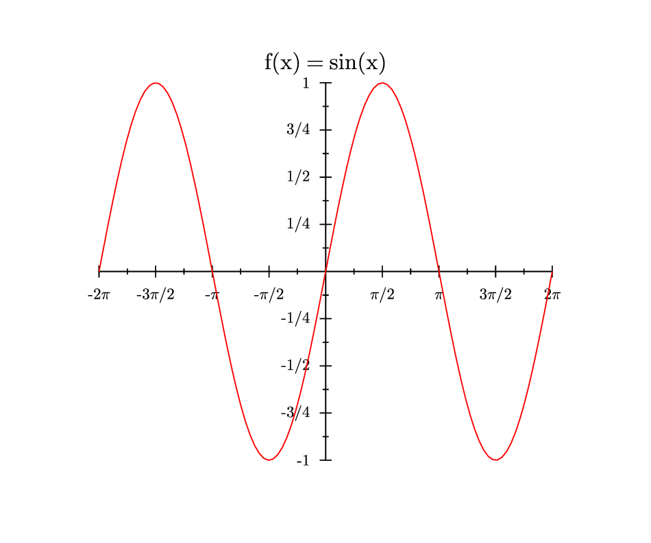
title "f(x) = sin(x)"
xaxis min -2*pi max 2*pi ftick -2*pi dticks pi/2 format "pi"
yaxis dticks 0.25 format "frac"
let d1 = sin(x)
d1 line color red
end graph
sine-approx.gle
sine-approx.gle
size 11 8
! Based on example by Pascal B.
include "graphutil.gle"
set texlabels 1
begin graph
scale auto
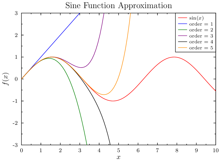
title "Sine Function Approximation"
xtitle "$x$"
xaxis min 0 max 10
yaxis min -3 max 3
ytitle "$f(x)$"
key pos tr hei 0.25
let d100 = sin(x)
let d101 = x
d100 line color autocolor(1) key "$\sin(x)$"
d101 line color autocolor(2) key "order = $1$"
let d1 = x
factorial = 1
for order = 2 to 5
n = order-1
factorial = factorial*(2*n)*(2*n+1)
let d[order] = d[order-1]+(-1)^(n)*(x^(2*n+1))/factorial
d[order] line color autocolor(order+1) key "order = $"+num$(order)+"$"
next order
end graph
sqroot.gle
sqroot.gle
size 11 8
set texlabels 1
begin graph
scale auto
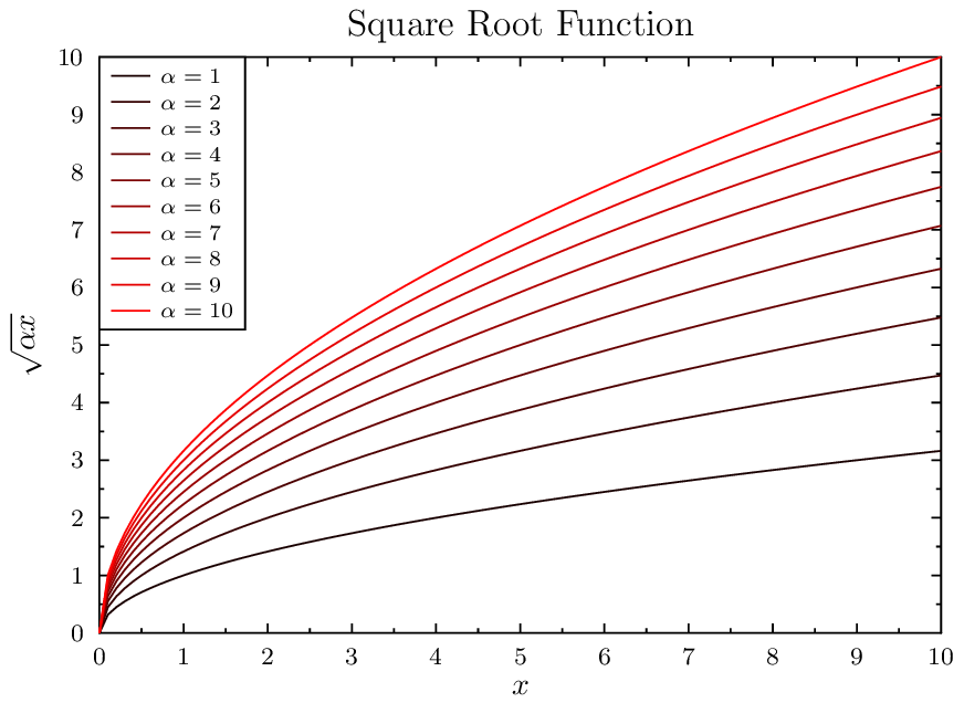
title "Square Root Function"
xtitle "$x$"
ytitle "$\sqrt{\alpha x}$"
key pos tl hei 0.25
for alpha = 1 to 10
let d[alpha] = sqrt(alpha*x) from 0 to 10
d[alpha] line color rgb(alpha/10,0,0) key "$\alpha = "+num$(alpha)+"$"
next alpha
end graph
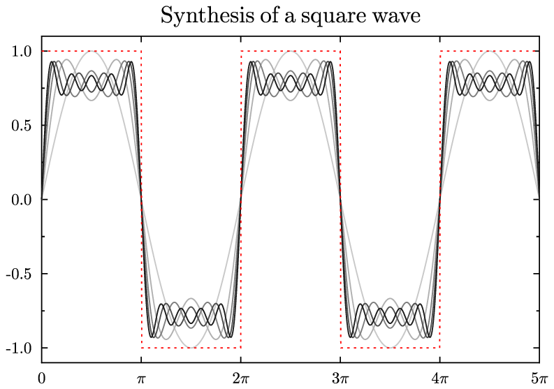
square.gle
square.gle
! Example of combining datasets

size 10 7

set font texcmr
begin graph
   scale auto
   title "Synthesis of a square wave"
   yaxis min -1.1 max 1.1
   xaxis min 0    max 5*pi dticks pi format "pi"
   xsubticks off
   let d1  = sin(x)   step 0.02        ! The fundamental sine wave
   let d2  = sin(3*x) step 0.02        ! Various harmonics over
   let d3  = sin(5*x) step 0.02        ! the fundamental
   let d4  = sin(7*x) step 0.02
   let d5  = sin(9*x) step 0.02
   let d20 = sgn(d1)                   ! The square wave
   let d10 = d1+(1/3)*d2               ! We take linear combinations
   let d11 = d10+(1/5)*d3              ! of the various frequencies
   let d12 = d11+(1/7)*d4
   let d13 = d12+(1/9)*d5
   d1  line color gray10               ! These could also be plotted
   d10 line color gray20               ! in different colors or line
   d11 line color gray40               ! styles to make the difference
   d12 line color gray60               ! clearer. A key may also help
   d13 line color gray80
   d20 line color red lstyle 2
end graph
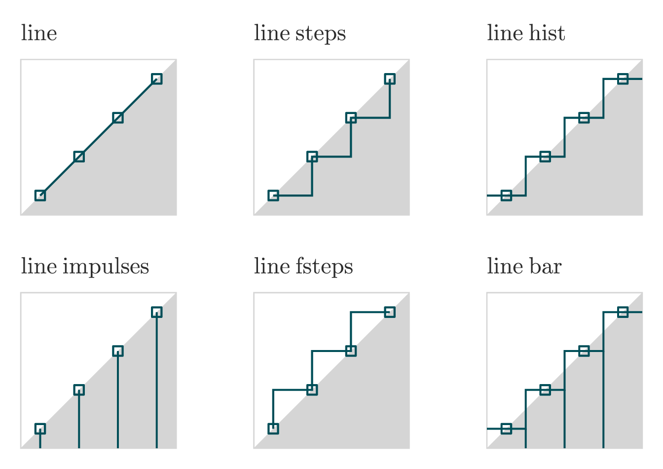
steps.gle
steps.gle
! Demo about line steps.
! Author: Francois Tonneau

size 17 12

set font ss hei 0.6

! GLE lets us define subroutines that work like procedures or functions. Here we
! will use a subroutine to create a panel with a triangle, a title, and a line
! drawn in a given style. Our 'panel' procedure will have three parameters: two
! numeric ('left' and 'bottom') and one string ('style$'). In GLE, the name of
! a string parameter or variable must end with a dollar sign.

sub panel left bottom style$
    amove left bottom
    begin origin
        set color #d5d5d5
        set lwidth 0.03
        box 4 4

        ! A 'begin path ... end path' block allows us to draw and/or fill an
        ! arbitrary closed region. Here the region will be a triangle filled
        ! with the #d5d5d5 color. We only need to define two sides of the
        ! triangle, as GLE automatically connects the beginning and end of a
        ! path when doing the filling. If we had wanted a filled triangle with
        ! a visible contour, however, we should have added 'stroke' after 'fill'
        ! ('begin path fill #d5d5d5 stroke'), and we should have closed the path
        ! explicity with the 'closepath' command.

        amove 0 0
        begin path fill #d5d5d5
            rline  4  4
            rline  0 -4
        end path

        ! Using GLE's string concatenation operator ('+'), we compose the title
        ! of our panel from "line " and the style$ parameter:

        amove 0 4.5
        set color #2c2c2c
        write "line "+style$

        ! We use a graph block with hidden axes ('axis off') to draw a line
        ! inside the panel. 'fullsize' means that the plot will take up its
        ! full assigned area; ticks and labels, if any, will lie outside.

        amove 0 0
        begin graph
            size 4 4
            fullsize
            xaxis min 0.5 max 4.5
            yaxis min 0.5 max 4.5
            axis  off

            ! To plot the line, we define a custom dataset with the 'let dn =
            ! x-expression from ... to ... step ...' syntax:

            let d1 = x from 1 to 4 step 1

            ! We use the 'if ... then ... else if ... end if' syntax to plot
            ! our custom dataset. The drawing command differs, depending on
            ! the value of style$:

            d1 color #004e58 lwidth 0.05 marker square msize 0.35
            if style$ = "" then
                d1 line
            else if style$ = "steps" then
                d1 line steps
            else if style$ = "hist" then
                d1 line hist
            else if style$ = "impulses" then
                d1 line impulses
            else if style$ = "fsteps" then
                d1 line fsteps
            else if style$ = "bar" then
                d1 line bar
            end if
        end graph

    end origin
end sub

! Now is the time to use our 'panel' subroutine:

panel 0.5  6.5 ""
panel 6.5  6.5 "steps"
panel 12.5 6.5 "hist"
panel 0.5  0.5 "impulses"
panel 6.5  0.5 "fsteps"
panel 12.5 0.5 "bar"

! Done. We have learned about line/step styles in GLE, 'begin path ... end
! path' blocks, subroutines, and if-then-else control flow.
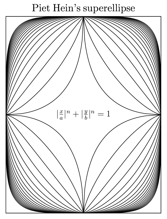
super-ellipse.gle
super-ellipse.gle
! Graphical representation of Piet Hein's superellipse

size 8 10.5

set cap round just tc hei 0.5 font rm

amove 4 5
begin origin                     ! Sets the origin of the ellipse at (10,9)
   a = 3.75; b = 4.75            ! a and b represent the excentricity of the ellipse
   begin clip
      amove -a -b                ! Draws the box that represents the limit as n tends to
      begin path clip stroke
         box 2*a 2*b             ! infinity
      end path
      for n=0.5 to 5 step 0.25   ! n is the exponent of the ellipse
         for i=0 to 360          ! Calculates the radial distance from the x and y
            ang = torad(i)
            c = abs(cos(ang))
            s = abs(sin(ang))
            ax = (c/a)^n         ! ax is the projection of the radial coordinate along the x axis
            ay = (s/b)^n         ! ay is the same along the y axis
            z = 1/(ax+ay)^(1/n)
            if i = 0 then
               amove z*cos(ang) z*sin(ang)
            else
               aline z*cos(ang) z*sin(ang)
            end if
         next i
      next n
   end clip
end origin

amove pagewidth()/2 pageheight()-0.15
write "Piet Hein's superellipse"

set just cc
amove pagewidth()/2 5
tex "\large $|\frac{x}{a}|^n + |\frac{y}{b}|^n = 1$"
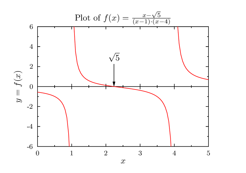
texgraph.gle
texgraph.gle
size 10 7

set texlabels 1 titlescale 1
begin graph
   title   "Plot of $f(x) = \frac{x-\sqrt{5}}{(x-1)\cdot(x-4)}$"
   ytitle  "$y = f(x)$"
   x0title "$x$"
   xaxis min 0 max 5 dticks 1 offset 0 symticks
   yaxis min -6 max 6
   let d1 = (x-sqrt(5))/((x-1)*(x-4)) from 0 to 5
   d1 line color red
   xlabels off
   x0labels on
   x0axis on symticks off
   x2axis on symticks off
end graph

set just bc
amove xg(sqrt(5)) yg(2.5)
tex "$\sqrt{5}$" add 0.1 name sq5b

amove pointx(sq5b.bc) pointy(sq5b.bc)
aline xg(sqrt(5)) yg(0) arrow end